pacman::p_load(tmap, SpatialAcc, sf, ggstatsplot, reshape2, tidyverse)In-Class Exercise 10: Modelling Geographical Accessibility
Alt: Hands-On Exercise 10
Imports
Packages
Geospatial
mpsz <- st_read(dsn = "data/geospatial", layer = "MP14_SUBZONE_NO_SEA_PL")Reading layer `MP14_SUBZONE_NO_SEA_PL' from data source
`/Users/michelle/Desktop/IS415/shelle-mim/IS415-GAA/Hands-on_Exercise/Wk11/data/geospatial'
using driver `ESRI Shapefile'
Simple feature collection with 323 features and 15 fields
Geometry type: MULTIPOLYGON
Dimension: XY
Bounding box: xmin: 2667.538 ymin: 15748.72 xmax: 56396.44 ymax: 50256.33
Projected CRS: SVY21hexagons <- st_read(dsn = "data/geospatial", layer = "hexagons") Reading layer `hexagons' from data source
`/Users/michelle/Desktop/IS415/shelle-mim/IS415-GAA/Hands-on_Exercise/Wk11/data/geospatial'
using driver `ESRI Shapefile'
Simple feature collection with 3125 features and 6 fields
Geometry type: POLYGON
Dimension: XY
Bounding box: xmin: 2667.538 ymin: 21506.33 xmax: 50010.26 ymax: 50256.33
Projected CRS: SVY21 / Singapore TMeldercare <- st_read(dsn = "data/geospatial", layer = "ELDERCARE") Reading layer `ELDERCARE' from data source
`/Users/michelle/Desktop/IS415/shelle-mim/IS415-GAA/Hands-on_Exercise/Wk11/data/geospatial'
using driver `ESRI Shapefile'
Simple feature collection with 120 features and 19 fields
Geometry type: POINT
Dimension: XY
Bounding box: xmin: 14481.92 ymin: 28218.43 xmax: 41665.14 ymax: 46804.9
Projected CRS: SVY21 / Singapore TMAspatial
ODMatrix <- read_csv("data/aspatial/OD_Matrix.csv", skip = 0)Data Wrangling
Geospatial
Update CRS information
mpsz <- st_transform(mpsz, 3414)
eldercare <- st_transform(eldercare, 3414)
hexagons <- st_transform(hexagons, 3414)
Cleaning and updating attribute fields of the geospatial data
eldercare <- eldercare %>%
  select(fid, ADDRESSPOS) %>%
  rename(destination_id = fid,
         postal_code = ADDRESSPOS) %>%
  mutate(capacity = 100) ## lazy method, by right this should be determined seperately for each eldercare

hexagons <- hexagons %>%
  select(fid) %>%
  rename(origin_id = fid) %>%
  mutate(demand = 100)
Aspatial
Tidy distance matrix
distmat <- ODMatrix %>%
  select(origin_id, destination_id, total_cost) %>%
  spread(destination_id, total_cost) %>% # similar to a pivot, but also slices the data to use only dest id as the pivot id
  select(c(-c('origin_id')))
distmat_km <- as.matrix(distmat/1000) # convert from m to kmCompute Dist Matrix
eldercare_coord <- st_coordinates(eldercare)
hexagon_coord <- st_coordinates(hexagons)
EucMatrox <- SpatialAcc::distance(hexagon_coord,
eldercare_coord,
type = "euclidean")Hansen’s Accessibility
Calculate
acc_Hansen <- data.frame(ac(hexagons$demand,
                            eldercare$capacity,
                            distmat_km,
                            #d0 = 50, # threshold of 50 km
                            power = 2,
family = "Hansen")) # can also change family for other tests, e.g. SAMcolnames(acc_Hansen) <- "accHansen"acc_Hansen <- tibble::as_tibble(acc_Hansen)hexagon_Hansen <- bind_cols(hexagons, acc_Hansen)Visualisation
mapex <- st_bbox(hexagons)tmap_mode("plot")
tm_shape(hexagon_Hansen,
bbox = mapex) +
tm_fill(col = "accHansen",
n = 10,
style = "quantile",
border.col = "black",
border.lwd = 1) +
tm_shape(eldercare) +
tm_symbols(size = 0.1) +
tm_layout(main.title = "Accessibility to eldercare: Hansen method",
main.title.position = "center",
main.title.size = 2,
legend.outside = FALSE,
legend.height = 0.45,
legend.width = 3.0,
legend.format = list(digits = 6),
legend.position = c("right", "top"),
frame = TRUE) +
tm_compass(type="8star", size = 2) +
tm_scale_bar(width = 0.15) +
tm_grid(lwd = 0.1, alpha = 0.5)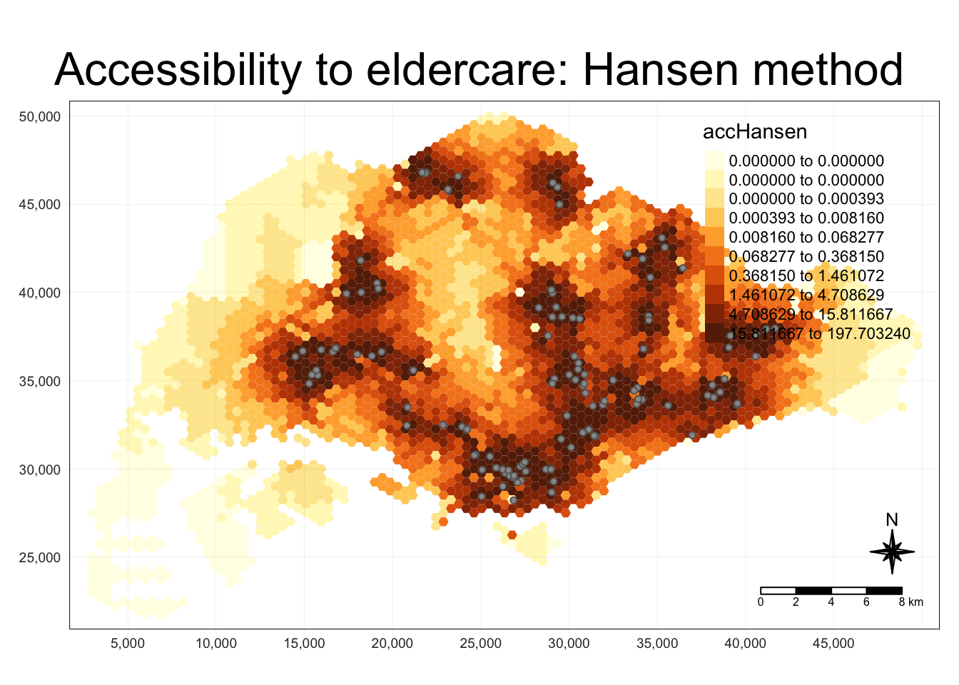
Statistical Visualisation
hexagon_Hansen <- st_join(hexagon_Hansen, mpsz,
join = st_intersects)ggplot(data=hexagon_Hansen,
aes(y = log(accHansen), # log transformation. if do not do, a lot of the distributions will be flat / 0
x= REGION_N)) +
geom_boxplot() +
geom_point(stat="summary",
fun.y="mean",
colour ="red",
size=2)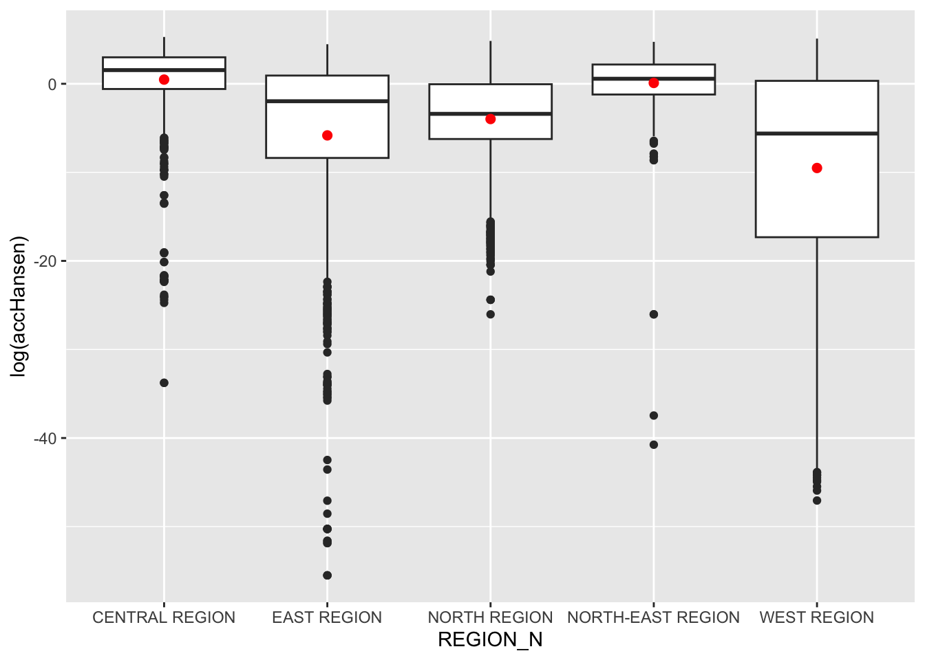
KD2SFCA Method
Calculate
acc_KD2SFCA <- data.frame(ac(hexagons$demand,
                            eldercare$capacity,
                            distmat_km,
                            d0 = 50,
                            power = 2,
                            family = "KD2SFCA"))

colnames(acc_KD2SFCA) <- "accKD2SFCA"
acc_KD2SFCA <- tibble::as_tibble(acc_KD2SFCA)
hexagon_KD2SFCA <- bind_cols(hexagons, acc_KD2SFCA)
Visualise
tmap_mode("plot")
tm_shape(hexagon_KD2SFCA,
         bbox = mapex) +
  tm_fill(col = "accKD2SFCA",
          n = 10,
          style = "quantile",
          border.col = "black",
          border.lwd = 1) +
tm_shape(eldercare) +
  tm_symbols(size = 0.1) +
  tm_layout(main.title = "Accessibility to eldercare: KD2SFCA method",
            main.title.position = "center",
            main.title.size = 2,
            legend.outside = FALSE,
            legend.height = 0.45,
            legend.width = 3.0,
            legend.format = list(digits = 6),
            legend.position = c("right", "top"),
            frame = TRUE) +
  tm_compass(type="8star", size = 2) +
  tm_scale_bar(width = 0.15) +
  tm_grid(lwd = 0.1, alpha = 0.5)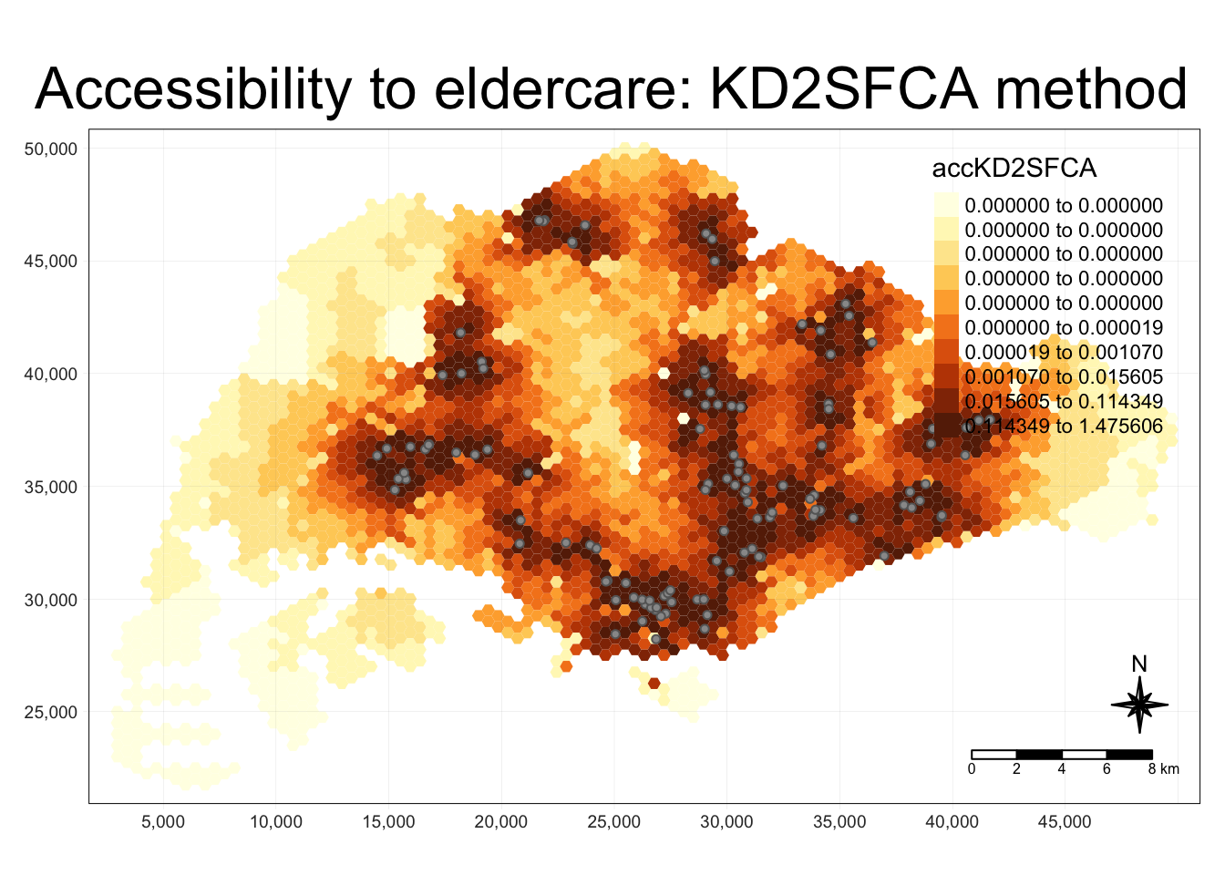
Statistical Visualisation
hexagon_KD2SFCA <- st_join(hexagon_KD2SFCA, mpsz,
                          join = st_intersects)

ggplot(data=hexagon_KD2SFCA,
       aes(y = accKD2SFCA,
           x= REGION_N)) +
  geom_boxplot() +
  geom_point(stat="summary",
             fun.y="mean",
             colour ="red",
             size=2)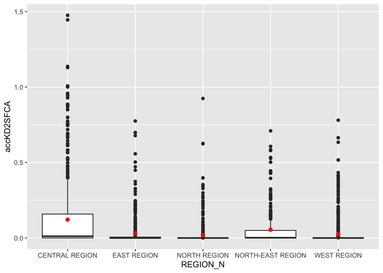
Spatial Accessibility Measure (SAM) Method
Compute
acc_SAM <- data.frame(ac(hexagons$demand,
                         eldercare$capacity,
                         distmat_km,
                         d0 = 50,
                         power = 2,
                         family = "SAM"))

colnames(acc_SAM) <- "accSAM"
acc_SAM <- tibble::as_tibble(acc_SAM)
hexagon_SAM <- bind_cols(hexagons, acc_SAM)
Visualise
tmap_mode("plot")
tm_shape(hexagon_SAM,
         bbox = mapex) +
  tm_fill(col = "accSAM",
          n = 10,
          style = "quantile",
          border.col = "black",
          border.lwd = 1) +
tm_shape(eldercare) +
  tm_symbols(size = 0.1) +
  tm_layout(main.title = "Accessibility to eldercare: SAM method",
            main.title.position = "center",
            main.title.size = 2,
            legend.outside = FALSE,
            legend.height = 0.45,
            legend.width = 3.0,
            legend.format = list(digits = 3),
            legend.position = c("right", "top"),
            frame = TRUE) +
  tm_compass(type="8star", size = 2) +
  tm_scale_bar(width = 0.15) +
  tm_grid(lwd = 0.1, alpha = 0.5)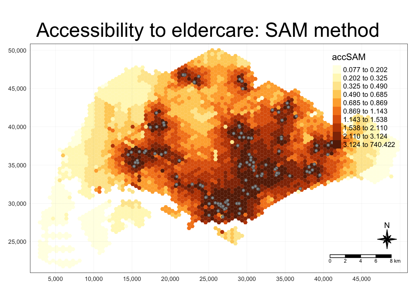
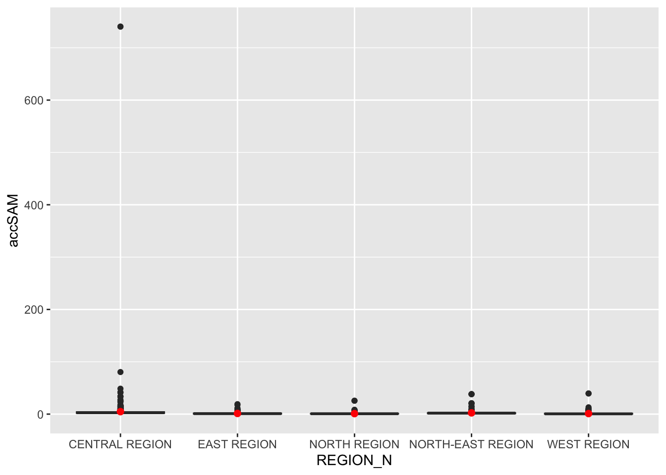
Statistical Visualise
hexagon_SAM <- st_join(hexagon_SAM, mpsz,
                       join = st_intersects)

ggplot(data=hexagon_SAM,
       aes(y = accSAM,
           x= REGION_N)) +
  geom_boxplot() +
  geom_point(stat="summary",
             fun.y="mean",
             colour ="red",
             size=2)