pacman::p_load(sf, tidyverse, tmap, maptools, raster, spatstat, sfdep)Take-Home Exercise 1: Application of Spatial Point Pattern Analysis on Osun State, Nigeria
Background & Objective of the Exercise
In this exercise, we investigate the distribution and availability of Water Points and access to clean water in the state of Osun, Nigeria. This will be done through the application of various Spatial Point Pattern Analyses in order to discover the geographical distribution of functional and non-functional Water Points in Osun.
In this exercise, we will be using data from the global Water Point Data Exchange (WPdx) project.
Installing Packages & Importing the Data
Install Relevant Packages
For this exercise, we will be using the following packages:
sf for importing, managing, and processing geospatial data
tidyverse for performing data science tasks such as importing, wrangling and visualising data
tmap which provides functions for plotting cartographic quality static point patterns maps or interactive maps
maptools which provides a set of tools for manipulating geographic data
raster which reads, writes, manipulates, analyses and model of gridded spatial data
spatstat, for its wide range of useful functions for point pattern analysis, and
sfdep for performing geospatial data wrangling and local colocation quotient analysis
Import Geospatial Data
GeoBoundaries data set
geoNGA = st_read(dsn = "data/geospatial",
layer = "geoBoundaries-NGA-ADM2") %>%
st_transform(crs = 26392)Reading layer `geoBoundaries-NGA-ADM2' from data source
`/Users/michelle/Desktop/IS415/shelle-mim/IS415-GAA/Take-home_Exercise/TH1/data/geospatial'
using driver `ESRI Shapefile'
Simple feature collection with 774 features and 5 fields
Geometry type: MULTIPOLYGON
Dimension: XY
Bounding box: xmin: 2.668534 ymin: 4.273007 xmax: 14.67882 ymax: 13.89442
Geodetic CRS: WGS 84head(geoNGA, n=3)Simple feature collection with 3 features and 5 fields
Geometry type: MULTIPOLYGON
Dimension: XY
Bounding box: xmin: 538408.1 ymin: 116360.7 xmax: 1248985 ymax: 1079710
Projected CRS: Minna / Nigeria Mid Belt
shapeName Level shapeID shapeGroup shapeType
1 Aba North ADM2 NGA-ADM2-72505758B79815894 NGA ADM2
2 Aba South ADM2 NGA-ADM2-72505758B67905963 NGA ADM2
3 Abadam ADM2 NGA-ADM2-72505758B57073987 NGA ADM2
geometry
1 MULTIPOLYGON (((548795.5 11...
2 MULTIPOLYGON (((541412.3 12...
3 MULTIPOLYGON (((1248985 104...NGA data set
NGA <- st_read("data/geospatial/",
layer = "nga_admbnda_adm2") %>%
st_transform(crs = 26392) # transform to PCS of NigeriaReading layer `nga_admbnda_adm2' from data source
`/Users/michelle/Desktop/IS415/shelle-mim/IS415-GAA/Take-home_Exercise/TH1/data/geospatial'
using driver `ESRI Shapefile'
Simple feature collection with 774 features and 16 fields
Geometry type: MULTIPOLYGON
Dimension: XY
Bounding box: xmin: 2.668534 ymin: 4.273007 xmax: 14.67882 ymax: 13.89442
Geodetic CRS: WGS 84head(NGA, n=3)Simple feature collection with 3 features and 16 fields
Geometry type: MULTIPOLYGON
Dimension: XY
Bounding box: xmin: 538408.1 ymin: 116360.7 xmax: 1248985 ymax: 1079710
Projected CRS: Minna / Nigeria Mid Belt
Shape_Leng Shape_Area ADM2_EN ADM2_PCODE ADM2_REF ADM2ALT1EN ADM2ALT2EN
1 0.2370744 0.001523921 Aba North NG001001 Aba North <NA> <NA>
2 0.2624772 0.003531104 Aba South NG001002 Aba South <NA> <NA>
3 3.0753158 0.326867840 Abadam NG008001 Abadam <NA> <NA>
ADM1_EN ADM1_PCODE ADM0_EN ADM0_PCODE date validOn validTo
1 Abia NG001 Nigeria NG 2016-11-29 2019-04-17 <NA>
2 Abia NG001 Nigeria NG 2016-11-29 2019-04-17 <NA>
3 Borno NG008 Nigeria NG 2016-11-29 2019-04-17 <NA>
SD_EN SD_PCODE geometry
1 Abia South NG00103 MULTIPOLYGON (((548795.5 11...
2 Abia South NG00103 MULTIPOLYGON (((547286.1 11...
3 Borno North NG00802 MULTIPOLYGON (((1248985 104...Import Aspatial Data
wp_nga <- read_csv("data/aspatial/WPDEx.csv") %>%
filter(`#clean_country_name` == "Nigeria") #remove irrelavent data, keep the data smallData Processing & Cleaning
Convert Aspatial to Geospatial
# use log and lat to make georeference col
wp_nga$Geometry = st_as_sfc(wp_nga$`New Georeferenced Column`)
head(wp_nga)# A tibble: 6 × 71
row_id #sour…¹ #lat_…² #lon_…³ #repo…⁴ #stat…⁵ #wate…⁶ #wate…⁷ #wate…⁸ #wate…⁹
<dbl> <chr> <dbl> <dbl> <chr> <chr> <chr> <chr> <chr> <chr>
1 429068 GRID3 7.98 5.12 08/29/… Unknown <NA> <NA> Tapsta… Tapsta…
2 222071 Federa… 6.96 3.60 08/16/… Yes Boreho… Well Mechan… Mechan…
3 160612 WaterA… 6.49 7.93 12/04/… Yes Boreho… Well Hand P… Hand P…
4 160669 WaterA… 6.73 7.65 12/04/… Yes Boreho… Well <NA> <NA>
5 160642 WaterA… 6.78 7.66 12/04/… Yes Boreho… Well Hand P… Hand P…
6 160628 WaterA… 6.96 7.78 12/04/… Yes Boreho… Well Hand P… Hand P…
# … with 61 more variables: `#facility_type` <chr>,
# `#clean_country_name` <chr>, `#clean_adm1` <chr>, `#clean_adm2` <chr>,
# `#clean_adm3` <chr>, `#clean_adm4` <chr>, `#install_year` <dbl>,
# `#installer` <chr>, `#rehab_year` <lgl>, `#rehabilitator` <lgl>,
# `#management_clean` <chr>, `#status_clean` <chr>, `#pay` <chr>,
# `#fecal_coliform_presence` <chr>, `#fecal_coliform_value` <dbl>,
# `#subjective_quality` <chr>, `#activity_id` <chr>, `#scheme_id` <chr>, …wp_sf <- st_sf(wp_nga, crs=4326)
wp_sfSimple feature collection with 95008 features and 70 fields
Geometry type: POINT
Dimension: XY
Bounding box: xmin: 2.707441 ymin: 4.301812 xmax: 14.21828 ymax: 13.86568
Geodetic CRS: WGS 84
# A tibble: 95,008 × 71
row_id `#source` #lat_…¹ #lon_…² #repo…³ #stat…⁴ #wate…⁵ #wate…⁶ #wate…⁷
* <dbl> <chr> <dbl> <dbl> <chr> <chr> <chr> <chr> <chr>
1 429068 GRID3 7.98 5.12 08/29/… Unknown <NA> <NA> Tapsta…
2 222071 Federal Minis… 6.96 3.60 08/16/… Yes Boreho… Well Mechan…
3 160612 WaterAid 6.49 7.93 12/04/… Yes Boreho… Well Hand P…
4 160669 WaterAid 6.73 7.65 12/04/… Yes Boreho… Well <NA>
5 160642 WaterAid 6.78 7.66 12/04/… Yes Boreho… Well Hand P…
6 160628 WaterAid 6.96 7.78 12/04/… Yes Boreho… Well Hand P…
7 160632 WaterAid 7.02 7.84 12/04/… Yes Boreho… Well Hand P…
8 642747 Living Water … 7.33 8.98 10/03/… Yes Boreho… Well Mechan…
9 642456 Living Water … 7.17 9.11 10/03/… Yes Boreho… Well Hand P…
10 641347 Living Water … 7.20 9.22 03/28/… Yes Boreho… Well Hand P…
# … with 94,998 more rows, 62 more variables: `#water_tech_category` <chr>,
# `#facility_type` <chr>, `#clean_country_name` <chr>, `#clean_adm1` <chr>,
# `#clean_adm2` <chr>, `#clean_adm3` <chr>, `#clean_adm4` <chr>,
# `#install_year` <dbl>, `#installer` <chr>, `#rehab_year` <lgl>,
# `#rehabilitator` <lgl>, `#management_clean` <chr>, `#status_clean` <chr>,
# `#pay` <chr>, `#fecal_coliform_presence` <chr>,
# `#fecal_coliform_value` <dbl>, `#subjective_quality` <chr>, …Projection Transformation
# Transform to appropriate projected coordinate system of Nigeria
wp_sf <- wp_sf %>%
st_transform(crs = 26392)Data Cleaning
Select relevant cols
# Select relevant adm1 and adm2 cols (cols 3-4 and 8-9)
NGA <- NGA %>%
dplyr::select(c(3:4, 8:9))Check for and Remove Duplicate Names
NGA$ADM2_EN[duplicated(NGA$ADM2_EN)==TRUE][1] "Bassa" "Ifelodun" "Irepodun" "Nasarawa" "Obi" "Surulere"# Save duplicated LGA names
duplicated_LGA <- NGA$ADM2_EN[duplicated(NGA$ADM2_EN)==TRUE]
# Find the indices of the duplicated LGAs
duplicated_indices <- which(NGA$ADM2_EN %in% duplicated_LGA)
# Edit names in at indices with duplicated names
for (ind in duplicated_indices) {
NGA$ADM2_EN[ind] <- paste(NGA$ADM2_EN[ind], NGA$ADM1_EN[ind], sep=", ")
}Data Wrangling
Extract Osun data
osun <- NGA %>%
filter(ADM1_EN %in%
c("Osun"))
qtm(osun)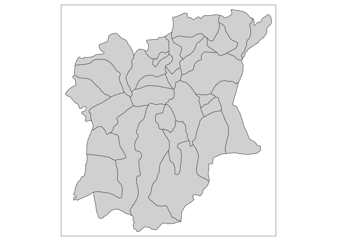
Exploratory Spatial Data Analysis
Derive Kernel Density Maps
Conversion to ppp data type
Before plotting our Kernel Density Maps, we first need to convert our data into the appropriate ppp data type.
# Convert sf to sp's spatial class
wp_functional_spatial <- as_Spatial(wp_functional_sf)
wp_nonfunctional_spatial <- as_Spatial(wp_nonfunctional_sf)
osun_spatial <- as_Spatial(osun)# Check spatial data type
wp_functional_spatialclass : SpatialPointsDataFrame
features : 52148
extent : 29322.63, 1218553, 33758.37, 1092629 (xmin, xmax, ymin, ymax)
crs : +proj=tmerc +lat_0=4 +lon_0=8.5 +k=0.99975 +x_0=670553.98 +y_0=0 +a=6378249.145 +rf=293.465 +towgs84=-92,-93,122,0,0,0,0 +units=m +no_defs
variables : 1
names : status_clean
min values : Functional
max values : Functional but not in use wp_nonfunctional_spatialclass : SpatialPointsDataFrame
features : 32204
extent : 28907.91, 1209690, 33736.93, 1092883 (xmin, xmax, ymin, ymax)
crs : +proj=tmerc +lat_0=4 +lon_0=8.5 +k=0.99975 +x_0=670553.98 +y_0=0 +a=6378249.145 +rf=293.465 +towgs84=-92,-93,122,0,0,0,0 +units=m +no_defs
variables : 1
names : status_clean
min values : Abandoned
max values : Non-Functional due to dry season osun_spatialclass : SpatialPolygonsDataFrame
features : 30
extent : 176503.2, 291043.8, 331434.7, 454520.1 (xmin, xmax, ymin, ymax)
crs : +proj=tmerc +lat_0=4 +lon_0=8.5 +k=0.99975 +x_0=670553.98 +y_0=0 +a=6378249.145 +rf=293.465 +towgs84=-92,-93,122,0,0,0,0 +units=m +no_defs
variables : 4
names : ADM2_EN, ADM2_PCODE, ADM1_EN, ADM1_PCODE
min values : Aiyedade, NG030001, Osun, NG030
max values : Osogbo, NG030030, Osun, NG030 # Convert to sp
wp_functional_sp <- as(wp_functional_spatial, "SpatialPoints")
wp_nonfunctional_sp <- as(wp_nonfunctional_spatial, "SpatialPoints")
osun_sp <- as(osun_spatial, "SpatialPolygons")wp_functional_spclass : SpatialPoints
features : 52148
extent : 29322.63, 1218553, 33758.37, 1092629 (xmin, xmax, ymin, ymax)
crs : +proj=tmerc +lat_0=4 +lon_0=8.5 +k=0.99975 +x_0=670553.98 +y_0=0 +a=6378249.145 +rf=293.465 +towgs84=-92,-93,122,0,0,0,0 +units=m +no_defs wp_functional_ppp <- as(wp_functional_sp, "ppp")
wp_nonfunctional_ppp <- as(wp_nonfunctional_sp, "ppp")plot(wp_functional_ppp)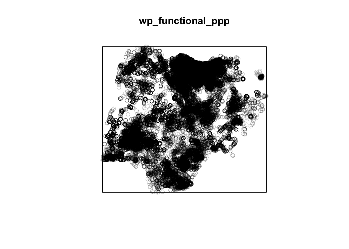
plot(wp_nonfunctional_ppp)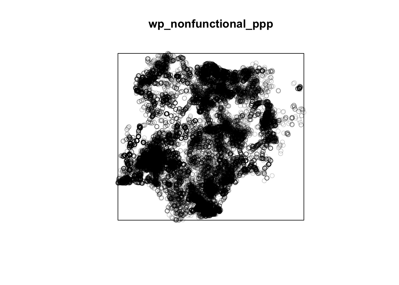
Check for/Deal with duplicated points
any(duplicated(wp_functional_ppp))[1] FALSEany(duplicated(wp_nonfunctional_ppp))[1] FALSESince there are no duplicated points, no further processing is needed.
Create Owin of Osun
Next, we create an owin object of Osun in order to bound our data within when representing our data on the map.
osun_owin <- as(osun_sp, "owin")plot(osun_owin)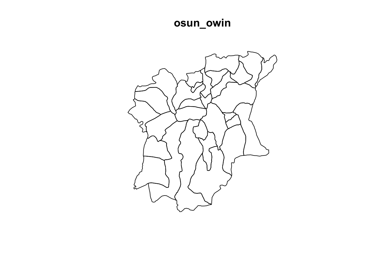
We can now use this owin of Osun to plot our Functional and Non-functional water point event data within.
wp_functional_osun_ppp = wp_functional_ppp[osun_owin]
wp_nonfunctional_osun_ppp = wp_nonfunctional_ppp[osun_owin]plot(wp_functional_osun_ppp)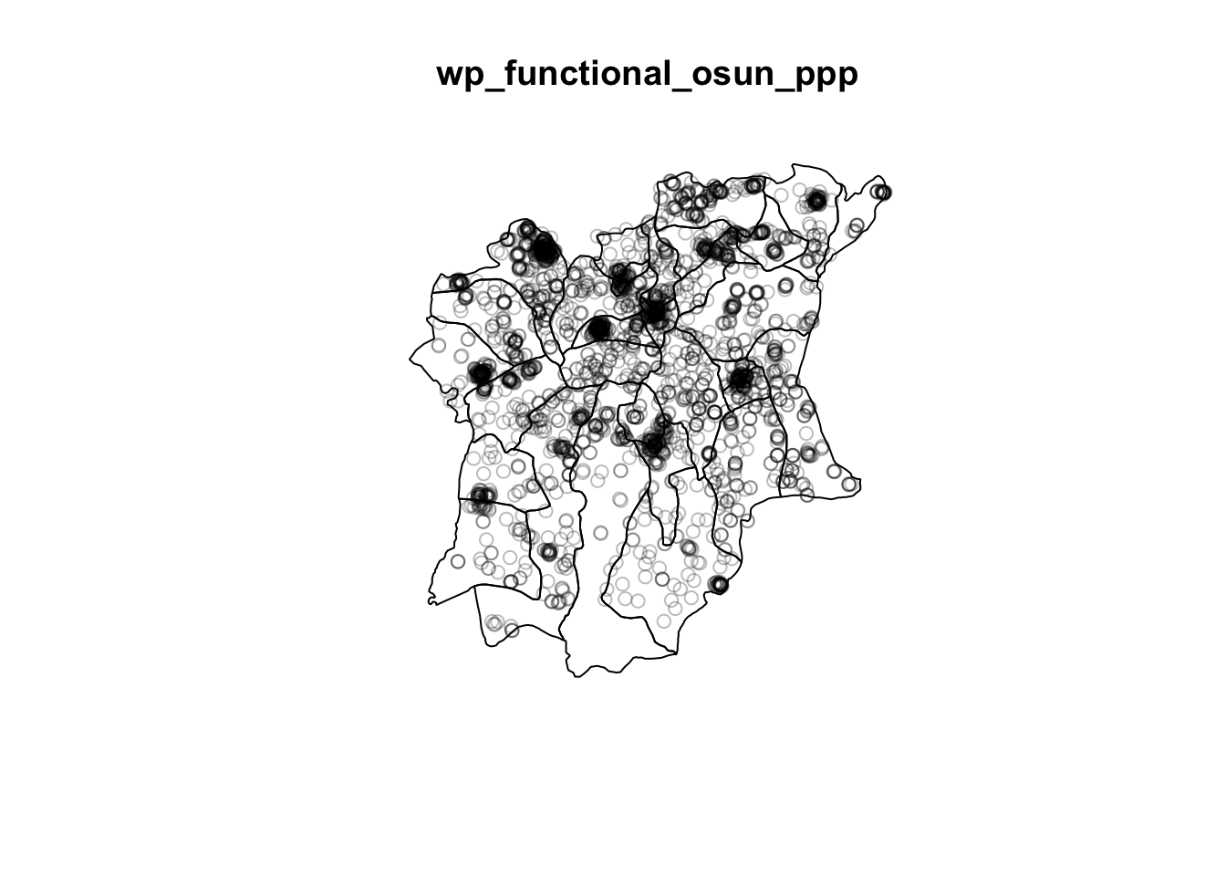
plot(wp_nonfunctional_osun_ppp)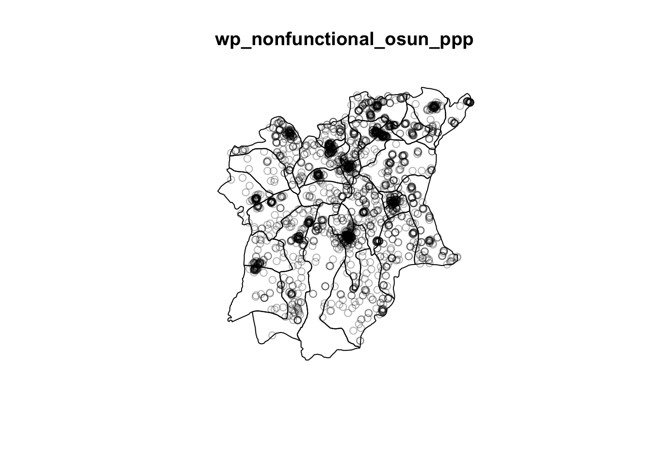
Kernel Density Estimation
With our data of Osun functional and non-functional water points assembled, we can now proceed to Kernel Density Estimation.
# Convert data to km as our unit of measurement
wp_func_osun_ppp_km <- rescale(wp_functional_osun_ppp, 1000, "km")
wp_nonfunc_osun_ppp_km <- rescale(wp_nonfunctional_osun_ppp, 1000, "km")For Kernel Density Estimation, there are multiple method in determining the bandwidth with which the calculation will be performed with. Below, we experiment with various automatic bandwith methods:
# Choosing automatic bandwith method
par(mfrow=c(2,2))
plot(density(wp_func_osun_ppp_km,
sigma=bw.CvL,
edge=TRUE,
kernel="gaussian"))
plot(density(wp_func_osun_ppp_km,
sigma=bw.scott,
edge=TRUE,
kernel="gaussian"))
plot(density(wp_func_osun_ppp_km,
sigma=bw.diggle,
edge=TRUE,
kernel="gaussian"))
plot(density(wp_func_osun_ppp_km,
sigma=bw.ppl,
edge=TRUE,
kernel="gaussian"))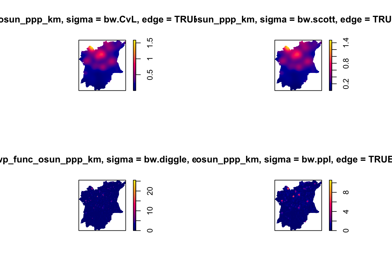
From these maps, I have choosen the bw.ppl method to be used. This is as from the visualisations we can see we appear to be working with predominately tight clusters, and bw.ppl and bw.diggle give more appropriate values when such is the case. I chose bw.ppl over bw.diggle as it shows up better than bw.diggle, which is slightly difficult to see in the visualisation above.
Now, we will choose our kernel method. The different kernel methods are demonstrated below:
# Choosing kernel method
par(mfrow=c(2,2))
plot(density(wp_func_osun_ppp_km,
sigma=bw.ppl,
edge=TRUE,
kernel="gaussian"),
main="Gaussian")
plot(density(wp_func_osun_ppp_km,
sigma=bw.ppl,
edge=TRUE,
kernel="epanechnikov"),
main="Epanechnikov")
plot(density(wp_func_osun_ppp_km,
sigma=bw.ppl,
edge=TRUE,
kernel="quartic"),
main="Quartic")
plot(density(wp_func_osun_ppp_km,
sigma=bw.ppl,
edge=TRUE,
kernel="disc"),
main="Disc")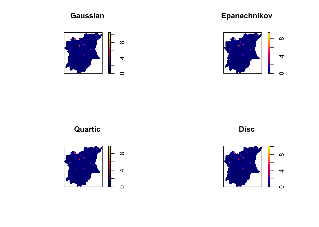
Since there are no significant differences observed across different kernels, we will use the Gaussian kernel, the default kernel method.
Lastly, to cover all bases, we shall try some adaptive bandwidth methods. Such methods are said to be better adapted to deal with skewed distributions of data.
par(mfrow=c(1,2))
# Try adaptive bandwith
plot( adaptive.density(wp_func_osun_ppp_km, method="voronoi"))
plot( adaptive.density(wp_func_osun_ppp_km, method="kernel"))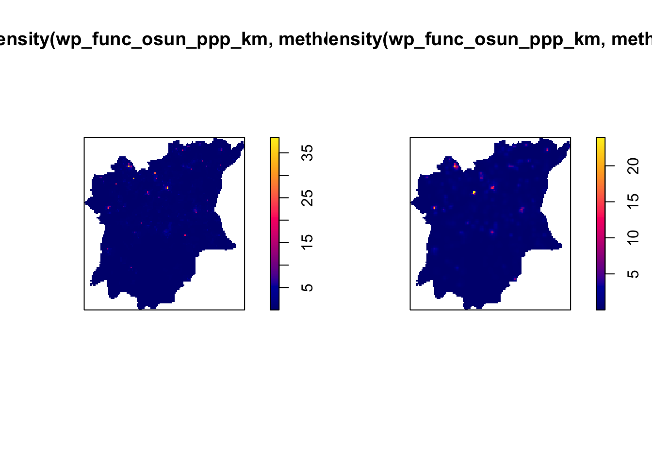
As we can see, adaptive bandwidth also does not give the best visualisations, so will stick to using the automatic bandwidth method, with bw.ppl and Gaussian kernel.
Hence, there are our final parameters of our Kernel Density Estimates will be as shown below:
kde_wp_func_bw_ppl <- density(wp_func_osun_ppp_km,
sigma=bw.ppl,
edge=TRUE,
kernel="gaussian")
kde_wp_nonfunc_bw_ppl <- density(wp_nonfunc_osun_ppp_km,
sigma=bw.ppl,
edge=TRUE,
kernel="gaussian")Final Kernel Density Estimation Maps
And finally, we shall plot our Kernel Density Maps.
par(mfrow=c(1,2))
plot(kde_wp_func_bw_ppl)
plot(kde_wp_nonfunc_bw_ppl)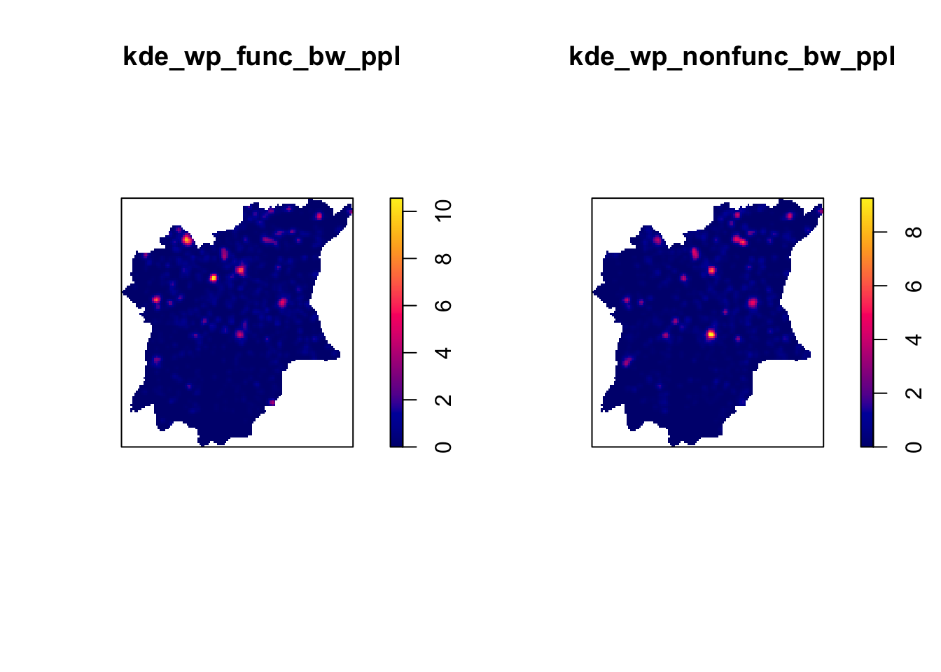
Display KDE Maps on OpenStreetMap
Convert to raster for tmap display
In order to display our KDE Maps on tmap, we would need to first convert out KDE Map to raster format.
# Convert to Gridded, then to raster
gridded_kde_wp_func_bw_ppl <- as.SpatialGridDataFrame.im(kde_wp_func_bw_ppl)
gridded_kde_wp_nonfunc_bw_ppl <- as.SpatialGridDataFrame.im(kde_wp_nonfunc_bw_ppl)
raster_kde_wp_func_bw_ppl <- raster(gridded_kde_wp_func_bw_ppl)
raster_kde_wp_nonfunc_bw_ppl <- raster(gridded_kde_wp_nonfunc_bw_ppl)
# Assign CRS info
projection(raster_kde_wp_func_bw_ppl) <- CRS("+init=EPSG:26392 +units=km")
projection(raster_kde_wp_nonfunc_bw_ppl) <- CRS("+init=EPSG:26392 +units=km")Display on tmap OpenStreetMap
Now that we have completed the transformation, we can display our maps on OpenStreetMap using tmap.
tmap_mode('view')
kde_func_wp <- tm_basemap("OpenStreetMap")+
tm_view(set.zoom.limits=c(9, 16)) +
tm_shape(raster_kde_wp_func_bw_ppl) +
tm_raster("v", palette="YlOrRd") +
tm_layout(legend.position = c("right", "bottom"), frame = FALSE)
kde_func_wpkde_nonfunc_wp <- tm_basemap("OpenStreetMap")+
tm_view(set.zoom.limits=c(9, 16)) +
tm_shape(raster_kde_wp_nonfunc_bw_ppl) +
tm_raster("v", palette="YlOrRd") +
tm_layout(legend.position = c("right", "bottom"), frame = FALSE)
kde_nonfunc_wpDescribe Spatial Patterns
Adding the LGA borders back on top of our KDE maps, we get:
tmap_mode('plot')
kde_func_wp +
tm_shape(osun) +
tm_borders() +
tm_text("ADM2_EN", size = 0.6) 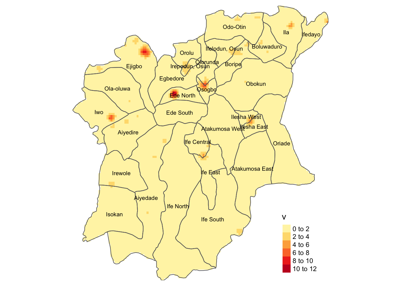
kde_nonfunc_wp +
tm_shape(osun) +
tm_borders() +
tm_text("ADM2_EN", size = 0.6) 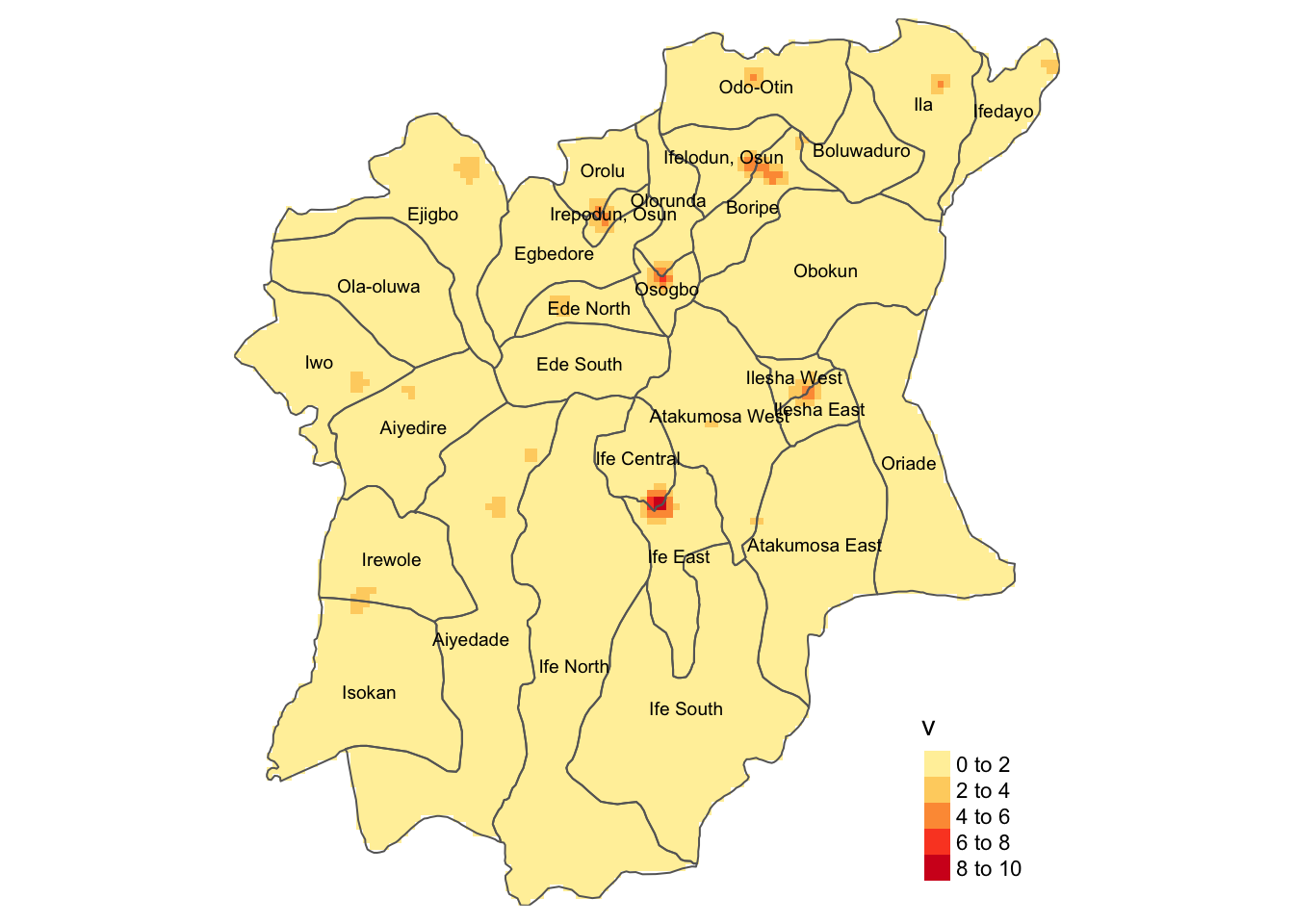
Benefit of Kernel Density Maps as a representation tool
As we can see from the two maps, it is very easy to pick out the areas with high density of water points in comparison to to point maps or choropleth maps. This is as the Kernel Density Estimate provides quantitative values of the concentration of points at a specific point, allowing for clean, uncluttered, and specific.
Kernel Density estimates also calculates the density of each area, allowing for a smoother estimate, and hence a better representation of the distribution of events on a map.
Spatial Pattern Analysis
From the plotted Kernel Density Maps, we can see there is a relatively high density of functional water points in the following LGAs, as denoted by the bright/dark red colors observed in the map:
Ejigbo
Ede North
Osogbo, and
Iwo
On the other hand, for non-functional water points in Osun, the high density lies primarily between the LGAs:
Ife Central, and
Ife East
We will do further analysis on some of these LGAs of interest in the next section.
Second-order Spatial Point Pattern Analysis
Formulate Null Hypothesis
Before carrying out our Second-order analysis on selected LGAs, we must first formulate our hypotheses to test our data against.
As such, below are the null and alternate hypotheses for the analysis on functional / non-functional water points respectively:
H0: The distribution of functional / nonfunctional water points in the given study area are randomly distributed.
H1: The distribution of functional / nonfunctional water points in the given study area are not randomly distributed.
Confidence level : 95%
Significance level (alpha) : 0.05
The null hypothesis will be rejected if p-value is smaller than alpha value of 0.05.
Perform test using G Function
Extracting Study Areas
Will be using the 2 most notable LGAs for Functional and Nonfunctional water points, which are:
For Functional: Ejigbo and Ede North
For Non-Functional: Ife Central and Ife East
We must now extract these 4 LGAs as owins, then populate them with the relavent Water Point data.
# Study Areas for Functional Water Points
ejigbo_owin <- NGA[NGA$ADM2_EN == "Ejigbo",] %>%
as('Spatial') %>%
as('SpatialPolygons') %>%
as('owin')
ede_north_owin <- NGA[NGA$ADM2_EN == "Ede North",] %>%
as('Spatial') %>%
as('SpatialPolygons') %>%
as('owin')
# Study Areas for NonFunctional Water Points
ife_central_owin <- NGA[NGA$ADM2_EN == "Ife Central",] %>%
as('Spatial') %>%
as('SpatialPolygons') %>%
as('owin')
ife_east_owin <- NGA[NGA$ADM2_EN == "Ife East",] %>%
as('Spatial') %>%
as('SpatialPolygons') %>%
as('owin')ejigbo_wp_func_ppp = rescale(wp_functional_ppp[ejigbo_owin], 1000, "km")
ede_north_wp_func_ppp = rescale(wp_functional_ppp[ede_north_owin], 1000, "km")
ife_central_wp_nonfunc_ppp = rescale(wp_nonfunctional_ppp[ife_central_owin], 1000, "km")
ife_east_wp_nonfunc_ppp = rescale(wp_nonfunctional_ppp[ife_east_owin], 1000, "km")par(mfrow=c(2,2))
plot(ejigbo_wp_func_ppp)
plot(ede_north_wp_func_ppp)
plot(ife_central_wp_nonfunc_ppp)
plot(ife_east_wp_nonfunc_ppp)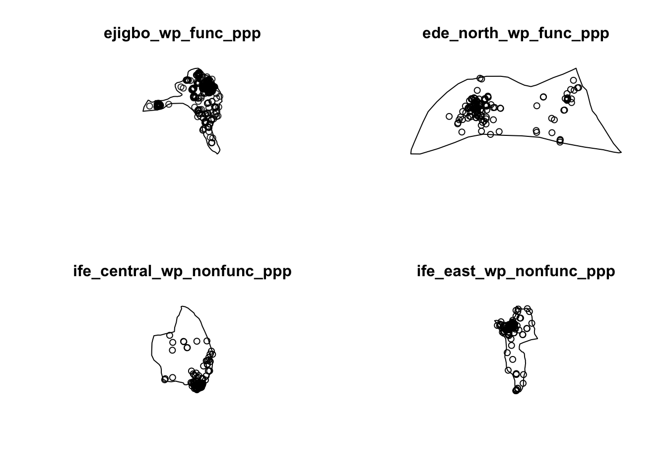
Calculating G Function
In this analysis, we will be using G Function in order to analyse the spatial distribution of water points in these 4 LGAs. The G function was chosen for this case as we are performing analysis on segments of our study area rather than the study area as a cumulative.
G_ejigbo = Gest(ejigbo_wp_func_ppp, correction = "border")
plot(G_ejigbo)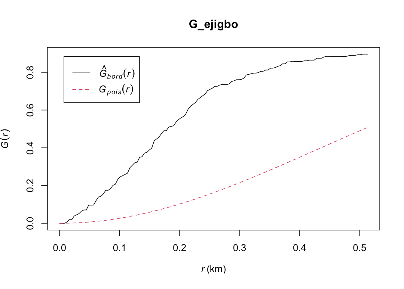
G_ejigbo.csr <- envelope(ejigbo_wp_func_ppp, Gest, nsim = 39)Generating 39 simulations of CSR ...
1, 2, 3, 4, 5, 6, 7, 8, 9, 10, 11, 12, 13, 14, 15, 16, 17, 18, 19, 20, 21, 22, 23, 24, 25, 26, 27, 28, 29, 30, 31, 32, 33, 34, 35, 36, 37, 38, 39.
Done.plot(G_ejigbo.csr)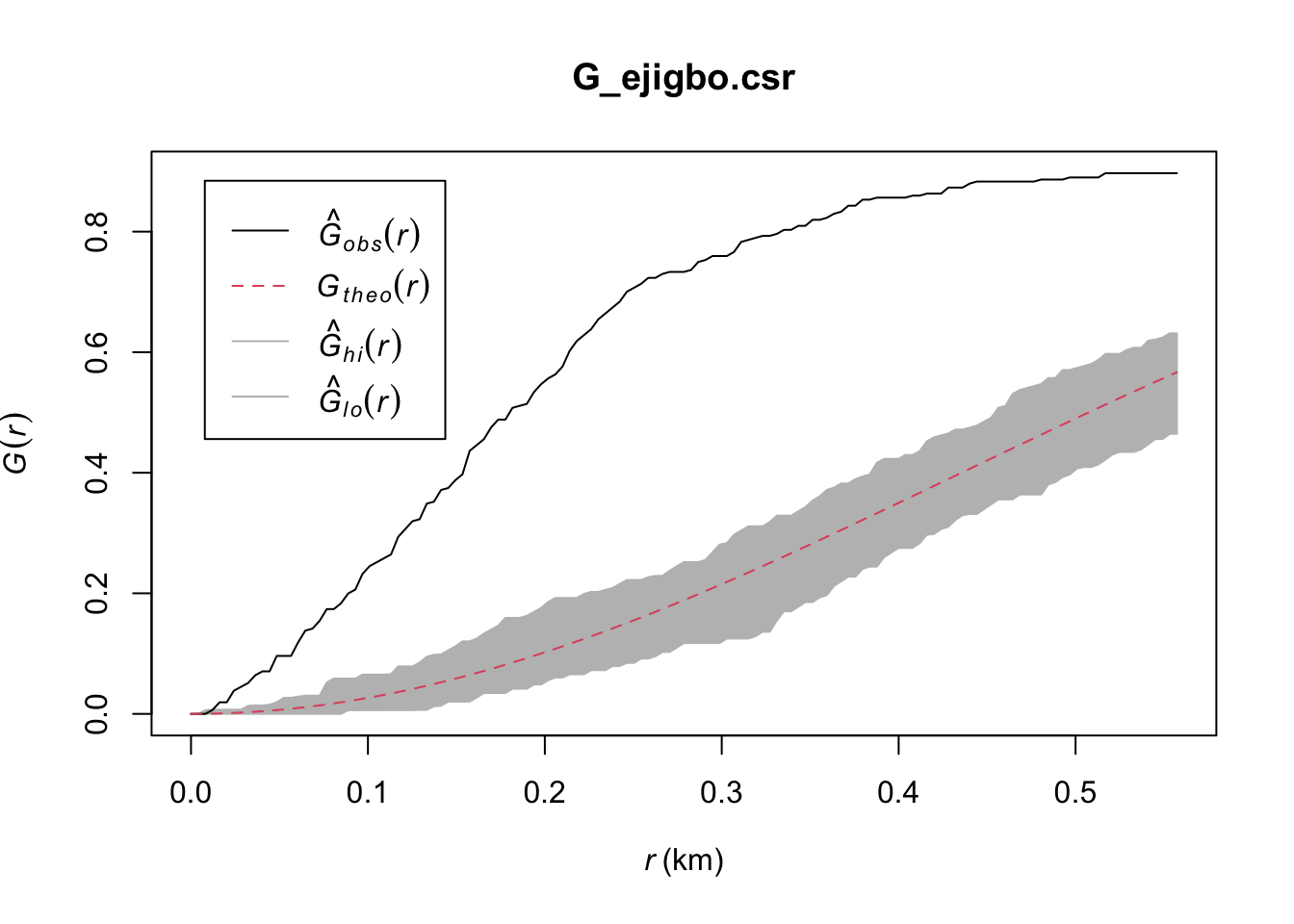
G_ede_north = Gest(ede_north_wp_func_ppp, correction = "border")
plot(G_ede_north)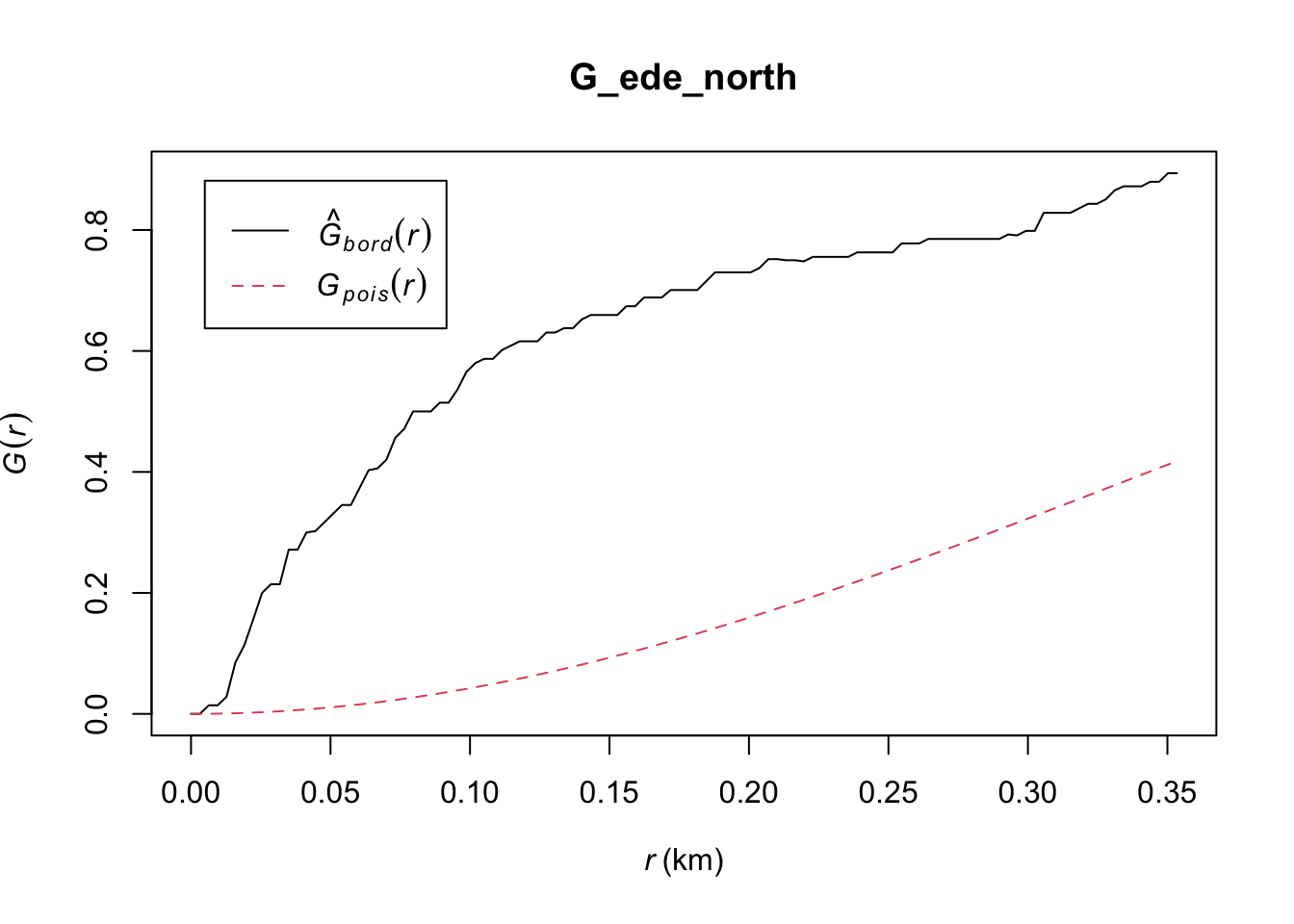
G_ede_north.csr <- envelope(ede_north_wp_func_ppp, Gest, nsim = 39)Generating 39 simulations of CSR ...
1, 2, 3, 4, 5, 6, 7, 8, 9, 10, 11, 12, 13, 14, 15, 16, 17, 18, 19, 20, 21, 22, 23, 24, 25, 26, 27, 28, 29, 30, 31, 32, 33, 34, 35, 36, 37, 38, 39.
Done.plot(G_ede_north.csr)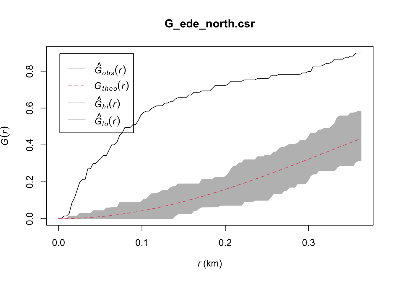
G_ife_central = Gest(ife_central_wp_nonfunc_ppp, correction = "border")
plot(G_ife_central)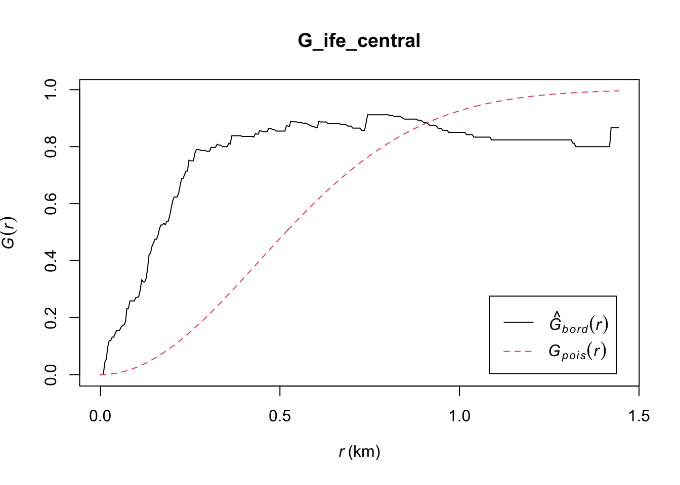
G_ife_central.csr <- envelope(ife_central_wp_nonfunc_ppp, Gest, nsim = 39)Generating 39 simulations of CSR ...
1, 2, 3, 4, 5, 6, 7, 8, 9, 10, 11, 12, 13, 14, 15, 16, 17, 18, 19, 20, 21, 22, 23, 24, 25, 26, 27, 28, 29, 30, 31, 32, 33, 34, 35, 36, 37, 38, 39.
Done.plot(G_ife_central.csr)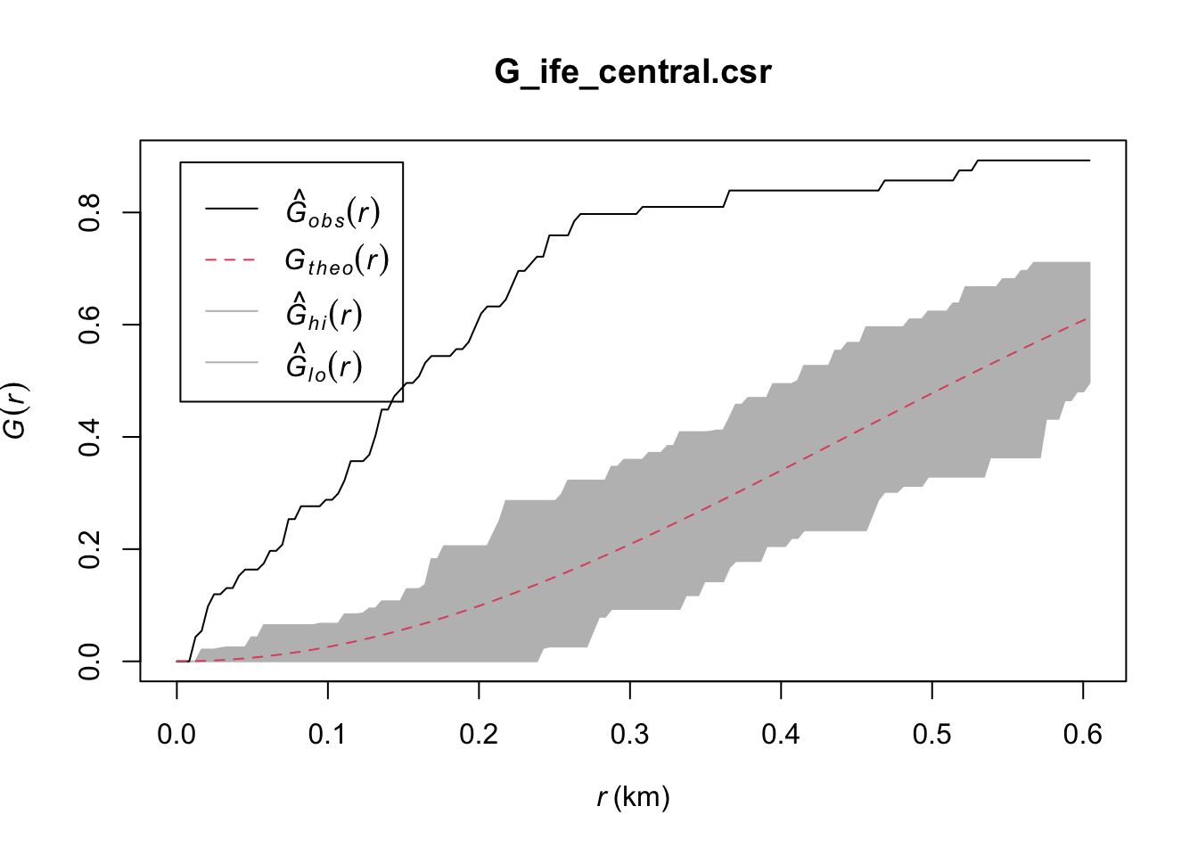
G_ife_east = Gest(ife_east_wp_nonfunc_ppp, correction = "border")
plot(G_ife_east)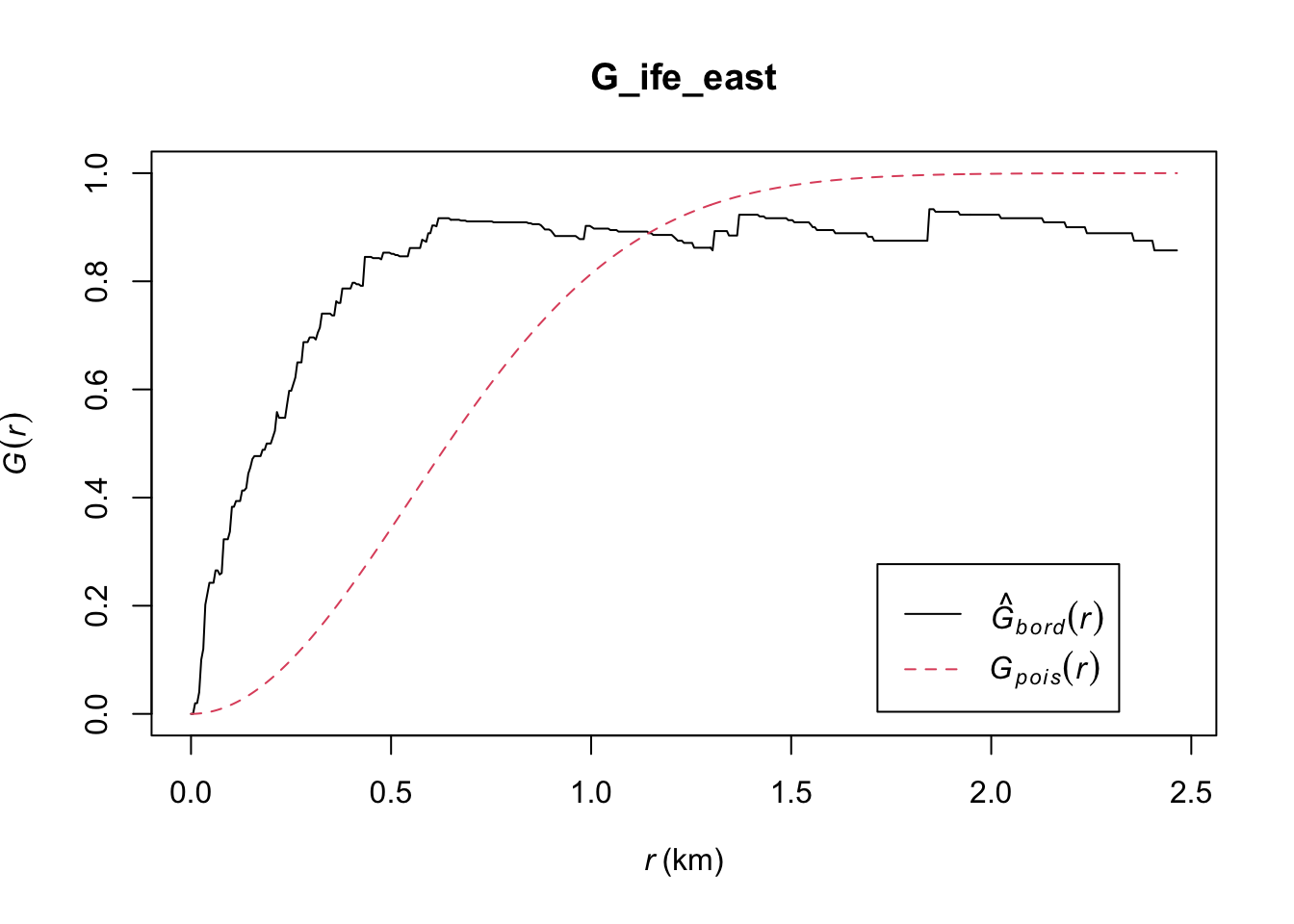
G_ife_east.csr <- envelope(ife_east_wp_nonfunc_ppp, Gest, nsim = 39)Generating 39 simulations of CSR ...
1, 2, 3, 4, 5, 6, 7, 8, 9, 10, 11, 12, 13, 14, 15, 16, 17, 18, 19, 20, 21, 22, 23, 24, 25, 26, 27, 28, 29, 30, 31, 32, 33, 34, 35, 36, 37, 38, 39.
Done.plot(G_ife_east.csr)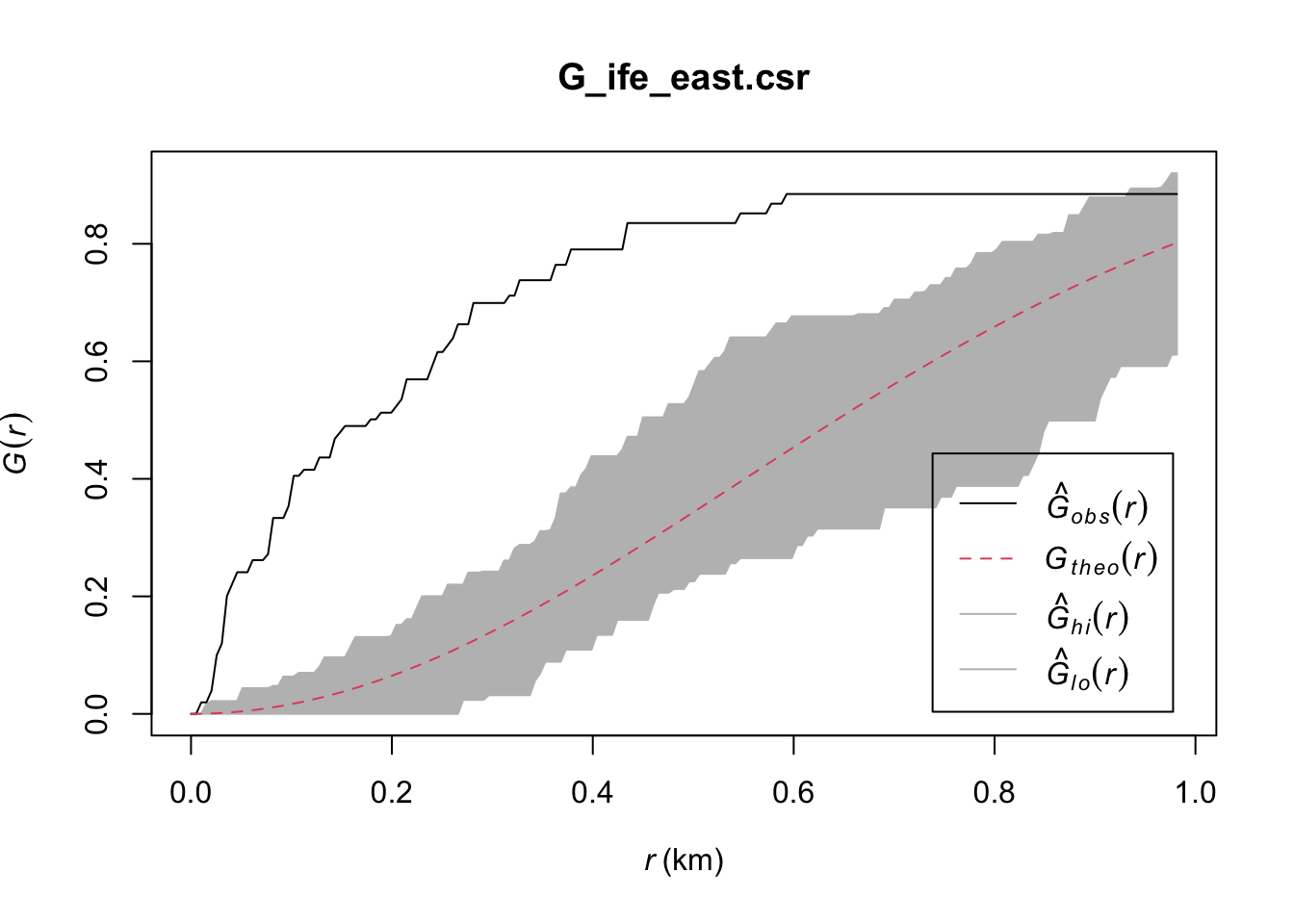
Second-Order Analysis Conclusion
From the graphs drawn, we can draw the following conclusions:
Ejigbo: The observed G(r) lies above the envelope at all plotted values of r, indicating that the Functional Water Points in Ejigbo are clustered. We can therefore reject the null hypothesis, and conclude that the Functional Water Points in Ejigbo are clustered with 95% confidence.
Ede North: Similarly, the observed G(r) lies above the envelope at all plotted values of r, indicating that the Functional Water Points in Ede North are clustered. We can therefore reject the null hypothesis, and conclude that the Functional Water Points in Ede North are clustered with 95% confidence.
Ife Central: Likewise, the observed G(r) lies above the envelope at all plotted values of r, indicating that the Non-Functional Water Points in Ife Central are clustered. We can therefore reject the null hypothesis, and conclude that the Non-Functional Water Points in Ife Central are clustered with 95% confidence.
Ife East: Lastly, we have Ife East, where the observed G(r) lies above the envelope, except at r > 0.925km (approximately). This indicates that the Non-Functional Water Points in Ife Central are clustered at values of r below 0.925km, and therefore for these values we can reject the null hypothesis, and conclude that the Non-Functional Water Points in Ife East at r < 0.925km are clustered with 95% confidence.
Spatial Correlation Analysis
Formulate Null Hypothesis and Alternative Hypothesis
Moving on to Spatial Correlation Analysis of Functional and Non-Functional Water Points in Osun, we will be testing the hypotheses as shown below:
H0: The Functional Water Points in Osun are not co-located with the Non-Functional Water Points in Osun.
H1: The Functional Water Points in Osun are co-located with the Non-Functional Water Points in Osun.
Confidence level : 95%
Significance level (alpha) : 0.05
The null hypothesis will be rejected if p-value is smaller than alpha value of 0.05.
Perform Local Colocation Quotient Analysis
Proprocessing to Osun data
In order to carry out our co-location analysis, we first need to assemble the relevant Osun Functional and Non-Functional Water point data.
# Re-select wp sf data
wp_sf_osun <- wp_sf %>%
st_intersection(osun) %>%
rename(status_clean = 'X.status_clean') %>%
rename(country_name = 'X.clean_country_name') %>%
rename(adm1 = 'X.clean_adm1') %>%
dplyr::select(status_clean, country_name, adm1) %>%
mutate(status_clean = replace_na(
status_clean, "unknown"
))
# Filter out non-osun data
wp_sf_osun <- wp_sf_osun %>% filter(adm1 %in%
c("Osun"))
# Create col to catagorise functional and non functional water points
wp_sf_osun <- wp_sf_osun %>%
mutate(`func_status` = case_when(
`status_clean` %in% c("Functional",
"Functional but not in use",
"Functional but needs repair") ~
"Functional",
`status_clean` %in% c("Abandoned/Decommissioned",
"Non-Functional due to dry season",
"Non-Functional",
"Abandoned",
"Non functional due to dry season") ~
"Non-Functional",
`status_clean` == "Unknown" ~ "Unknown"))
glimpse(wp_sf_osun)Rows: 5,322
Columns: 5
$ status_clean <chr> "Functional but needs repair", "Functional", "Functional"…
$ country_name <chr> "Nigeria", "Nigeria", "Nigeria", "Nigeria", "Nigeria", "N…
$ adm1 <chr> "Osun", "Osun", "Osun", "Osun", "Osun", "Osun", "Osun", "…
$ Geometry <POINT [m]> POINT (212810 386707.6), POINT (212202 349210.1), P…
$ func_status <chr> "Functional", "Functional", "Functional", "Functional", "…We can now plot the processed data to visualise the sf data we will be working with:
tmap_mode("view")
tm_shape(osun) +
tm_polygons() +
tm_shape(wp_sf_osun)+
tm_dots(col = "func_status",
size = 0.01,
border.col = "black",
border.lwd = 0.5) +
tm_view(set.zoom.limits = c(9, 16))Calculate Local Colocation Quotients
In order to compute the LCLQ, we first need to prepare the nearest neighbour list, kernel weights, and vector list, as done below:
# Prepare nearest neighbours list
nb <- include_self(
st_knn(st_geometry(wp_sf_osun), 6))
# Compute kernel weights
wt <- st_kernel_weights(nb,
wp_sf_osun,
"gaussian",
adaptive = TRUE)# Prepare vectors
Fuctional_vector <- wp_sf_osun %>%
filter(func_status == "Functional")
A <- Fuctional_vector$func_status
Non_Functional_vector <- wp_sf_osun %>%
filter(func_status == "Non-Functional")
B <- Non_Functional_vector$func_statusWith the relevant components prepared, we can now calculate the LCLQ values for each Functional Water Point, complete with the Complete Spatial Randomness Test.
LCLQ <- local_colocation(A, B, nb, wt, 49)In order to plot these values, we then join the output of the LCLQ through cbind().
LCLQ_osun <- cbind(wp_sf_osun, LCLQ)We can now plot the LCLQ values for analysis, with statistically significant LCLQ values that have a p-value of less than 0.05 highlighted in red:
tmap_mode("view")
osun_LCLQ_map <- tm_shape(osun) +
tm_polygons() +
tm_shape(LCLQ_osun)+
tm_dots(col = "Non.Functional",
size = 0.02,
border.col = "black",
border.lwd = 0.5,
alpha=0.5,
palette=c("red", "grey")) +
tm_view(set.zoom.limits = c(9, 16))
osun_LCLQ_mapConclusion
tmap_mode("plot")
osun_LCLQ_map +
tm_shape(osun) +
tm_borders() +
tm_text("ADM2_EN", size = 0.6) 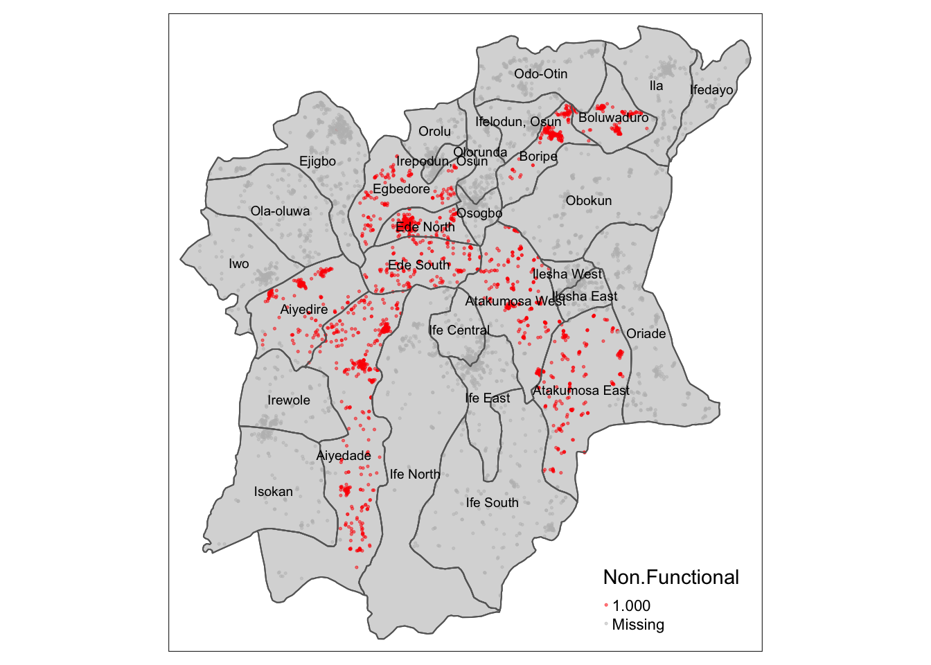
From this analysis, we can see that there indeed there is indeed some correlation between the location of Functional and Non-Functional water points in certain LGAs in Osun, most notably Boluwaduro, Boripe, Egbedore, Ede North, Ede South, Alyedire, Alyedade, Atakumosa West, and Atakumosa East, where the highlighted points are concentrated.
Upon examining the data more closely, it is observed that all the statistically significant points from the Complete Spatial Randomness Test, as highlighted in red, all have a Local Colocation Quotient of <1. Thus, for these points, we can reject the null hypothesis, and conclude that these Functional Water Points are indeed co-located with their surrounding Non-Functional Water Points with a 95% confidence. As for the nature of this correlation, from the LCLQ of <1, we can say that these Functional Water Points are less likely to have Non-Functional Water points in their neighbourhood. We can therefore infer that the LGA listed above, which have the majority of highlighted points, have a less than proportional number of Non-Functional Water Points for each Functional Water Point.