pacman::p_load(maptools, sf, raster, spatstat, tmap)In-Class Exercise 4: Spatial Point Patterns Analysis
Alt: Hands-On Exercise 4 & 5 - Spatial Point Patterns Analysis
Import Relevant Packages
Spatial Data Wrangling
# Import childcare spatial data
childcare_sf <- st_read("data/child-care-services-geojson.geojson") %>%
st_transform(crs = 3414)Reading layer `child-care-services-geojson' from data source
`/Users/michelle/Desktop/IS415/shelle-mim/IS415-GAA/Hands-on_Exercise/Wk4/data/child-care-services-geojson.geojson'
using driver `GeoJSON'
Simple feature collection with 1545 features and 2 fields
Geometry type: POINT
Dimension: XYZ
Bounding box: xmin: 103.6824 ymin: 1.248403 xmax: 103.9897 ymax: 1.462134
z_range: zmin: 0 zmax: 0
Geodetic CRS: WGS 84# Import coastal spatial data
sg_sf <- st_read(dsn = "data", layer="CostalOutline")Reading layer `CostalOutline' from data source
`/Users/michelle/Desktop/IS415/shelle-mim/IS415-GAA/Hands-on_Exercise/Wk4/data'
using driver `ESRI Shapefile'
Simple feature collection with 60 features and 4 fields
Geometry type: POLYGON
Dimension: XY
Bounding box: xmin: 2663.926 ymin: 16357.98 xmax: 56047.79 ymax: 50244.03
Projected CRS: SVY21# Import ura spatial data
mpsz_sf <- st_read(dsn = "data",
layer = "MP14_SUBZONE_WEB_PL")Reading layer `MP14_SUBZONE_WEB_PL' from data source
`/Users/michelle/Desktop/IS415/shelle-mim/IS415-GAA/Hands-on_Exercise/Wk4/data'
using driver `ESRI Shapefile'
Simple feature collection with 323 features and 15 fields
Geometry type: MULTIPOLYGON
Dimension: XY
Bounding box: xmin: 2667.538 ymin: 15748.72 xmax: 56396.44 ymax: 50256.33
Projected CRS: SVY21Assign correct CRS
sg_sf <- st_transform(sg_sf, 3414)
st_geometry(sg_sf)Geometry set for 60 features
Geometry type: POLYGON
Dimension: XY
Bounding box: xmin: 2663.926 ymin: 16357.98 xmax: 56047.79 ymax: 50244.03
Projected CRS: SVY21 / Singapore TM
First 5 geometries:mpsz_sf <- st_transform(mpsz_sf, 3414)
st_geometry(mpsz_sf)Geometry set for 323 features
Geometry type: MULTIPOLYGON
Dimension: XY
Bounding box: xmin: 2667.538 ymin: 15748.72 xmax: 56396.44 ymax: 50256.33
Projected CRS: SVY21 / Singapore TM
First 5 geometries:st_geometry(childcare_sf)Geometry set for 1545 features
Geometry type: POINT
Dimension: XYZ
Bounding box: xmin: 11203.01 ymin: 25667.6 xmax: 45404.24 ymax: 49300.88
z_range: zmin: 0 zmax: 0
Projected CRS: SVY21 / Singapore TM
First 5 geometries:All data is now in SVY21.
Mapping
# Static map of chilcares
tmap_mode("plot")
tm_shape(mpsz_sf) +
tm_polygons() +
tm_shape(childcare_sf) +
tm_dots(size = 0.002)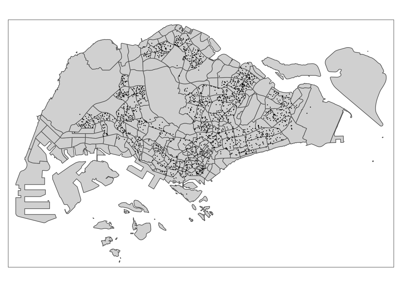
# Interactive Map
tmap_mode('view')
tm_basemap("OpenStreetMap")+
tm_view(set.zoom.limits=c(11, 16)) +
tm_shape(childcare_sf)+
tm_dots(alpha=0.5)tmap_mode('plot')Geospatial Data Wrangling
# Convert sf data to sp spatial class
childcare <- as_Spatial(childcare_sf)
mpsz <- as_Spatial(mpsz_sf)
sg <- as_Spatial(sg_sf)# Display info
list(childcare)[[1]]
class : SpatialPointsDataFrame
features : 1545
extent : 11203.01, 45404.24, 25667.6, 49300.88 (xmin, xmax, ymin, ymax)
crs : +proj=tmerc +lat_0=1.36666666666667 +lon_0=103.833333333333 +k=1 +x_0=28001.642 +y_0=38744.572 +ellps=WGS84 +towgs84=0,0,0,0,0,0,0 +units=m +no_defs
variables : 2
names : Name, Description
min values : kml_1, <center><table><tr><th colspan='2' align='center'><em>Attributes</em></th></tr><tr bgcolor="#E3E3F3"> <th>ADDRESSBLOCKHOUSENUMBER</th> <td></td> </tr><tr bgcolor=""> <th>ADDRESSBUILDINGNAME</th> <td></td> </tr><tr bgcolor="#E3E3F3"> <th>ADDRESSPOSTALCODE</th> <td>018989</td> </tr><tr bgcolor=""> <th>ADDRESSSTREETNAME</th> <td>1, MARINA BOULEVARD, #B1 - 01, ONE MARINA BOULEVARD, SINGAPORE 018989</td> </tr><tr bgcolor="#E3E3F3"> <th>ADDRESSTYPE</th> <td></td> </tr><tr bgcolor=""> <th>DESCRIPTION</th> <td></td> </tr><tr bgcolor="#E3E3F3"> <th>HYPERLINK</th> <td></td> </tr><tr bgcolor=""> <th>LANDXADDRESSPOINT</th> <td>0</td> </tr><tr bgcolor="#E3E3F3"> <th>LANDYADDRESSPOINT</th> <td>0</td> </tr><tr bgcolor=""> <th>NAME</th> <td>THE LITTLE SKOOL-HOUSE INTERNATIONAL PTE. LTD.</td> </tr><tr bgcolor="#E3E3F3"> <th>PHOTOURL</th> <td></td> </tr><tr bgcolor=""> <th>ADDRESSFLOORNUMBER</th> <td></td> </tr><tr bgcolor="#E3E3F3"> <th>INC_CRC</th> <td>08F73931F4A691F4</td> </tr><tr bgcolor=""> <th>FMEL_UPD_D</th> <td>20200826094036</td> </tr><tr bgcolor="#E3E3F3"> <th>ADDRESSUNITNUMBER</th> <td></td> </tr></table></center>
max values : kml_999, <center><table><tr><th colspan='2' align='center'><em>Attributes</em></th></tr><tr bgcolor="#E3E3F3"> <th>ADDRESSBLOCKHOUSENUMBER</th> <td></td> </tr><tr bgcolor=""> <th>ADDRESSBUILDINGNAME</th> <td></td> </tr><tr bgcolor="#E3E3F3"> <th>ADDRESSPOSTALCODE</th> <td>829646</td> </tr><tr bgcolor=""> <th>ADDRESSSTREETNAME</th> <td>200, PONGGOL SEVENTEENTH AVENUE, SINGAPORE 829646</td> </tr><tr bgcolor="#E3E3F3"> <th>ADDRESSTYPE</th> <td></td> </tr><tr bgcolor=""> <th>DESCRIPTION</th> <td>Child Care Services</td> </tr><tr bgcolor="#E3E3F3"> <th>HYPERLINK</th> <td></td> </tr><tr bgcolor=""> <th>LANDXADDRESSPOINT</th> <td>0</td> </tr><tr bgcolor="#E3E3F3"> <th>LANDYADDRESSPOINT</th> <td>0</td> </tr><tr bgcolor=""> <th>NAME</th> <td>RAFFLES KIDZ @ PUNGGOL PTE LTD</td> </tr><tr bgcolor="#E3E3F3"> <th>PHOTOURL</th> <td></td> </tr><tr bgcolor=""> <th>ADDRESSFLOORNUMBER</th> <td></td> </tr><tr bgcolor="#E3E3F3"> <th>INC_CRC</th> <td>379D017BF244B0FA</td> </tr><tr bgcolor=""> <th>FMEL_UPD_D</th> <td>20200826094036</td> </tr><tr bgcolor="#E3E3F3"> <th>ADDRESSUNITNUMBER</th> <td></td> </tr></table></center> list(mpsz)[[1]]
class : SpatialPolygonsDataFrame
features : 323
extent : 2667.538, 56396.44, 15748.72, 50256.33 (xmin, xmax, ymin, ymax)
crs : +proj=tmerc +lat_0=1.36666666666667 +lon_0=103.833333333333 +k=1 +x_0=28001.642 +y_0=38744.572 +ellps=WGS84 +towgs84=0,0,0,0,0,0,0 +units=m +no_defs
variables : 15
names : OBJECTID, SUBZONE_NO, SUBZONE_N, SUBZONE_C, CA_IND, PLN_AREA_N, PLN_AREA_C, REGION_N, REGION_C, INC_CRC, FMEL_UPD_D, X_ADDR, Y_ADDR, SHAPE_Leng, SHAPE_Area
min values : 1, 1, ADMIRALTY, AMSZ01, N, ANG MO KIO, AM, CENTRAL REGION, CR, 00F5E30B5C9B7AD8, 16409, 5092.8949, 19579.069, 871.554887798, 39437.9352703
max values : 323, 17, YUNNAN, YSSZ09, Y, YISHUN, YS, WEST REGION, WR, FFCCF172717C2EAF, 16409, 50424.7923, 49552.7904, 68083.9364708, 69748298.792 list(sg)[[1]]
class : SpatialPolygonsDataFrame
features : 60
extent : 2663.926, 56047.79, 16357.98, 50244.03 (xmin, xmax, ymin, ymax)
crs : +proj=tmerc +lat_0=1.36666666666667 +lon_0=103.833333333333 +k=1 +x_0=28001.642 +y_0=38744.572 +ellps=WGS84 +towgs84=0,0,0,0,0,0,0 +units=m +no_defs
variables : 4
names : GDO_GID, MSLINK, MAPID, COSTAL_NAM
min values : 1, 1, 0, ISLAND LINK
max values : 60, 67, 0, SINGAPORE - MAIN ISLAND # Convert to generic sp object
childcare_sp <- as(childcare, "SpatialPoints")
sg_sp <- as(sg, "SpatialPolygons")childcare_spclass : SpatialPoints
features : 1545
extent : 11203.01, 45404.24, 25667.6, 49300.88 (xmin, xmax, ymin, ymax)
crs : +proj=tmerc +lat_0=1.36666666666667 +lon_0=103.833333333333 +k=1 +x_0=28001.642 +y_0=38744.572 +ellps=WGS84 +towgs84=0,0,0,0,0,0,0 +units=m +no_defs sg_spclass : SpatialPolygons
features : 60
extent : 2663.926, 56047.79, 16357.98, 50244.03 (xmin, xmax, ymin, ymax)
crs : +proj=tmerc +lat_0=1.36666666666667 +lon_0=103.833333333333 +k=1 +x_0=28001.642 +y_0=38744.572 +ellps=WGS84 +towgs84=0,0,0,0,0,0,0 +units=m +no_defs # convert to spatstat's ppp format
childcare_ppp <- as(childcare_sp, "ppp")
childcare_pppPlanar point pattern: 1545 points
window: rectangle = [11203.01, 45404.24] x [25667.6, 49300.88] unitsplot(childcare_ppp)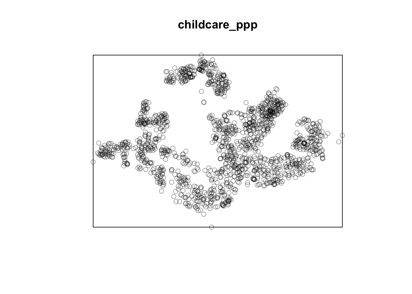
# statistics
summary(childcare_ppp)Planar point pattern: 1545 points
Average intensity 1.91145e-06 points per square unit
*Pattern contains duplicated points*
Coordinates are given to 3 decimal places
i.e. rounded to the nearest multiple of 0.001 units
Window: rectangle = [11203.01, 45404.24] x [25667.6, 49300.88] units
(34200 x 23630 units)
Window area = 808287000 square units# check for duplicated points (warning also appears in summary)
any(duplicated(childcare_ppp))[1] TRUE# find number of duiplicated points
# multiplicity() shows all points
sum(multiplicity(childcare_ppp) > 1)[1] 128# observe duplicated points (higher opacity spots on the map)
tmap_mode('view')
tm_shape(childcare) +
tm_dots(alpha=0.4,
size=0.05)tmap_mode('plot')Methods of Removing duplicate points
#1: Delete duplicated points => but removes useful data
#2: Jittering: add small perturbation so duplicate points are not in same place
childcare_ppp_jit <- rjitter(childcare_ppp,
retry=TRUE,
nsim=1,
drop=TRUE)any(duplicated(childcare_ppp_jit))[1] FALSE#3: Make each point unique, then attached duplicates as marks (attributes of the points) => needs analytical techniques to take into account marks
Creating owin object
Used to create a geographical area to confine analysis within
sg_owin <- as(sg_sp, "owin")plot(sg_owin)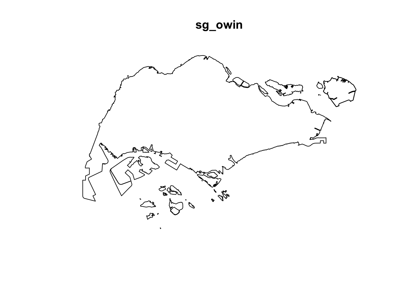
summary(sg_owin)Window: polygonal boundary
60 separate polygons (no holes)
vertices area relative.area
polygon 1 38 1.56140e+04 2.09e-05
polygon 2 735 4.69093e+06 6.27e-03
polygon 3 49 1.66986e+04 2.23e-05
polygon 4 76 3.12332e+05 4.17e-04
polygon 5 5141 6.36179e+08 8.50e-01
polygon 6 42 5.58317e+04 7.46e-05
polygon 7 67 1.31354e+06 1.75e-03
polygon 8 15 4.46420e+03 5.96e-06
polygon 9 14 5.46674e+03 7.30e-06
polygon 10 37 5.26194e+03 7.03e-06
polygon 11 53 3.44003e+04 4.59e-05
polygon 12 74 5.82234e+04 7.78e-05
polygon 13 69 5.63134e+04 7.52e-05
polygon 14 143 1.45139e+05 1.94e-04
polygon 15 165 3.38736e+05 4.52e-04
polygon 16 130 9.40465e+04 1.26e-04
polygon 17 19 1.80977e+03 2.42e-06
polygon 18 16 2.01046e+03 2.69e-06
polygon 19 93 4.30642e+05 5.75e-04
polygon 20 90 4.15092e+05 5.54e-04
polygon 21 721 1.92795e+06 2.57e-03
polygon 22 330 1.11896e+06 1.49e-03
polygon 23 115 9.28394e+05 1.24e-03
polygon 24 37 1.01705e+04 1.36e-05
polygon 25 25 1.66227e+04 2.22e-05
polygon 26 10 2.14507e+03 2.86e-06
polygon 27 190 2.02489e+05 2.70e-04
polygon 28 175 9.25904e+05 1.24e-03
polygon 29 1993 9.99217e+06 1.33e-02
polygon 30 38 2.42492e+04 3.24e-05
polygon 31 24 6.35239e+03 8.48e-06
polygon 32 53 6.35791e+05 8.49e-04
polygon 33 41 1.60161e+04 2.14e-05
polygon 34 22 2.54368e+03 3.40e-06
polygon 35 30 1.08382e+04 1.45e-05
polygon 36 327 2.16921e+06 2.90e-03
polygon 37 111 6.62927e+05 8.85e-04
polygon 38 90 1.15991e+05 1.55e-04
polygon 39 98 6.26829e+04 8.37e-05
polygon 40 415 3.25384e+06 4.35e-03
polygon 41 222 1.51142e+06 2.02e-03
polygon 42 107 6.33039e+05 8.45e-04
polygon 43 7 2.48299e+03 3.32e-06
polygon 44 17 3.28303e+04 4.38e-05
polygon 45 26 8.34758e+03 1.11e-05
polygon 46 177 4.67446e+05 6.24e-04
polygon 47 16 3.19460e+03 4.27e-06
polygon 48 15 4.87296e+03 6.51e-06
polygon 49 66 1.61841e+04 2.16e-05
polygon 50 149 5.63430e+06 7.53e-03
polygon 51 609 2.62570e+07 3.51e-02
polygon 52 8 7.82256e+03 1.04e-05
polygon 53 976 2.33447e+07 3.12e-02
polygon 54 55 8.25379e+04 1.10e-04
polygon 55 976 2.33447e+07 3.12e-02
polygon 56 61 3.33449e+05 4.45e-04
polygon 57 6 1.68410e+04 2.25e-05
polygon 58 4 9.45963e+03 1.26e-05
polygon 59 46 6.99702e+05 9.35e-04
polygon 60 13 7.00873e+04 9.36e-05
enclosing rectangle: [2663.93, 56047.79] x [16357.98, 50244.03] units
(53380 x 33890 units)
Window area = 748741000 square units
Fraction of frame area: 0.414# Combining point events with owin
childcareSG_ppp = childcare_ppp[sg_owin]
summary(childcareSG_ppp)Planar point pattern: 1545 points
Average intensity 2.063463e-06 points per square unit
*Pattern contains duplicated points*
Coordinates are given to 3 decimal places
i.e. rounded to the nearest multiple of 0.001 units
Window: polygonal boundary
60 separate polygons (no holes)
vertices area relative.area
polygon 1 38 1.56140e+04 2.09e-05
polygon 2 735 4.69093e+06 6.27e-03
polygon 3 49 1.66986e+04 2.23e-05
polygon 4 76 3.12332e+05 4.17e-04
polygon 5 5141 6.36179e+08 8.50e-01
polygon 6 42 5.58317e+04 7.46e-05
polygon 7 67 1.31354e+06 1.75e-03
polygon 8 15 4.46420e+03 5.96e-06
polygon 9 14 5.46674e+03 7.30e-06
polygon 10 37 5.26194e+03 7.03e-06
polygon 11 53 3.44003e+04 4.59e-05
polygon 12 74 5.82234e+04 7.78e-05
polygon 13 69 5.63134e+04 7.52e-05
polygon 14 143 1.45139e+05 1.94e-04
polygon 15 165 3.38736e+05 4.52e-04
polygon 16 130 9.40465e+04 1.26e-04
polygon 17 19 1.80977e+03 2.42e-06
polygon 18 16 2.01046e+03 2.69e-06
polygon 19 93 4.30642e+05 5.75e-04
polygon 20 90 4.15092e+05 5.54e-04
polygon 21 721 1.92795e+06 2.57e-03
polygon 22 330 1.11896e+06 1.49e-03
polygon 23 115 9.28394e+05 1.24e-03
polygon 24 37 1.01705e+04 1.36e-05
polygon 25 25 1.66227e+04 2.22e-05
polygon 26 10 2.14507e+03 2.86e-06
polygon 27 190 2.02489e+05 2.70e-04
polygon 28 175 9.25904e+05 1.24e-03
polygon 29 1993 9.99217e+06 1.33e-02
polygon 30 38 2.42492e+04 3.24e-05
polygon 31 24 6.35239e+03 8.48e-06
polygon 32 53 6.35791e+05 8.49e-04
polygon 33 41 1.60161e+04 2.14e-05
polygon 34 22 2.54368e+03 3.40e-06
polygon 35 30 1.08382e+04 1.45e-05
polygon 36 327 2.16921e+06 2.90e-03
polygon 37 111 6.62927e+05 8.85e-04
polygon 38 90 1.15991e+05 1.55e-04
polygon 39 98 6.26829e+04 8.37e-05
polygon 40 415 3.25384e+06 4.35e-03
polygon 41 222 1.51142e+06 2.02e-03
polygon 42 107 6.33039e+05 8.45e-04
polygon 43 7 2.48299e+03 3.32e-06
polygon 44 17 3.28303e+04 4.38e-05
polygon 45 26 8.34758e+03 1.11e-05
polygon 46 177 4.67446e+05 6.24e-04
polygon 47 16 3.19460e+03 4.27e-06
polygon 48 15 4.87296e+03 6.51e-06
polygon 49 66 1.61841e+04 2.16e-05
polygon 50 149 5.63430e+06 7.53e-03
polygon 51 609 2.62570e+07 3.51e-02
polygon 52 8 7.82256e+03 1.04e-05
polygon 53 976 2.33447e+07 3.12e-02
polygon 54 55 8.25379e+04 1.10e-04
polygon 55 976 2.33447e+07 3.12e-02
polygon 56 61 3.33449e+05 4.45e-04
polygon 57 6 1.68410e+04 2.25e-05
polygon 58 4 9.45963e+03 1.26e-05
polygon 59 46 6.99702e+05 9.35e-04
polygon 60 13 7.00873e+04 9.36e-05
enclosing rectangle: [2663.93, 56047.79] x [16357.98, 50244.03] units
(53380 x 33890 units)
Window area = 748741000 square units
Fraction of frame area: 0.414plot(childcareSG_ppp)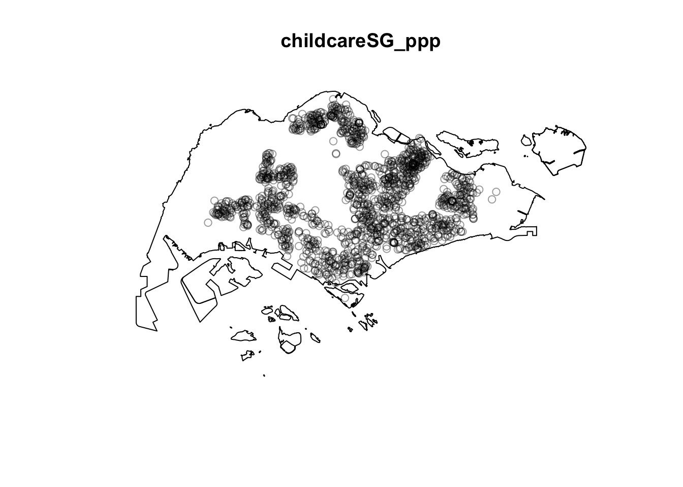
First-Order Spatial Point Pattern Analysis
Kernel Density Estimation
# bw.diggle = automatic bandwith selection. can also use bw.CvL(), bw.scott(), bw.ppl()
# kernel = smooting kernel/selected smoothing method (others: epanechnikov, quartic, disc)
kde_childcareSG_bw <- density(childcareSG_ppp,
sigma=bw.diggle,
edge=TRUE,
kernel="gaussian") plot(kde_childcareSG_bw)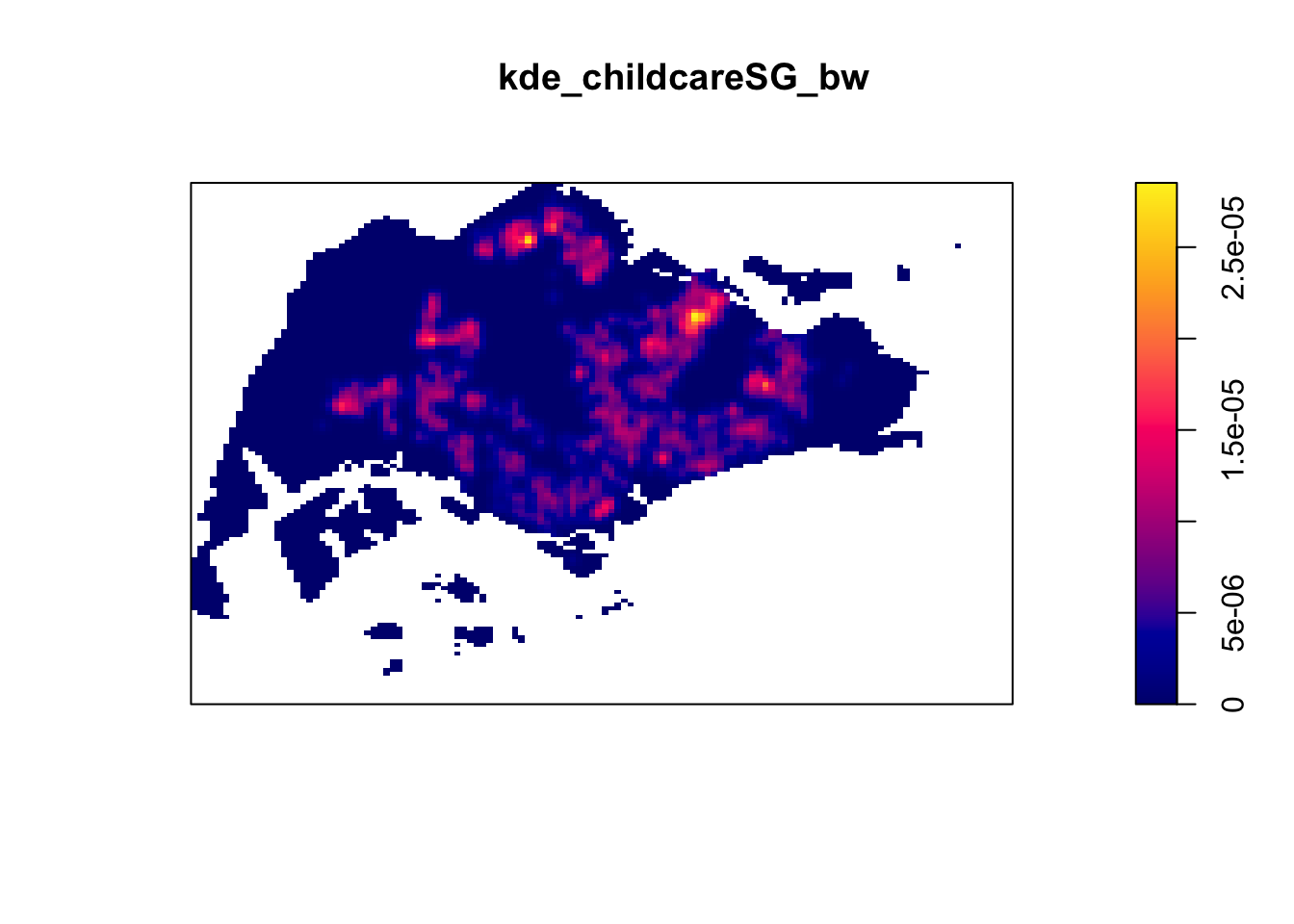
# Retrieve the bandwith used to computer kde layer
bw <- bw.diggle(childcareSG_ppp)
bw sigma
298.4095 # Rescaling KDE values (convert unit of measurement)
childcareSG_ppp.km <- rescale(childcareSG_ppp, 1000, "km")kde_childcareSG.bw <- density(childcareSG_ppp.km, sigma=bw.diggle, edge=TRUE, kernel="gaussian")
plot(kde_childcareSG.bw)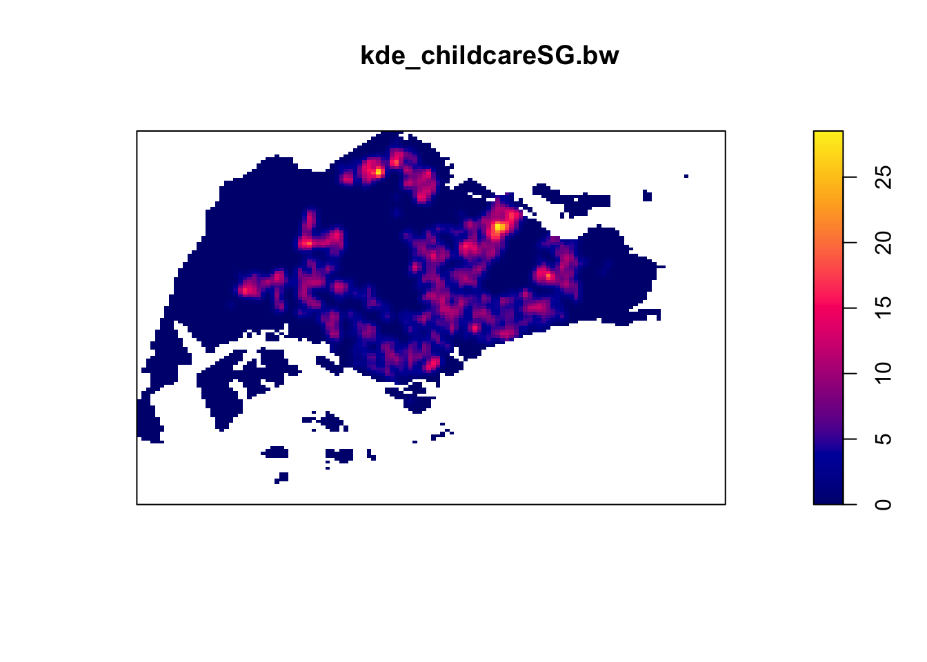
Other bandwidth calc methods:
bw.CvL(childcareSG_ppp.km) sigma
4.543278 bw.scott(childcareSG_ppp.km) sigma.x sigma.y
2.224898 1.450966 bw.ppl(childcareSG_ppp.km) sigma
0.3897114 bw.diggle(childcareSG_ppp.km) sigma
0.2984095 # Compare outputs of bw.diggle vs bw.ppl
kde_childcareSG.ppl <- density(childcareSG_ppp.km,
sigma=bw.ppl,
edge=TRUE,
kernel="gaussian")
par(mfrow=c(1,2))
plot(kde_childcareSG.bw, main = "bw.diggle")
plot(kde_childcareSG.ppl, main = "bw.ppl")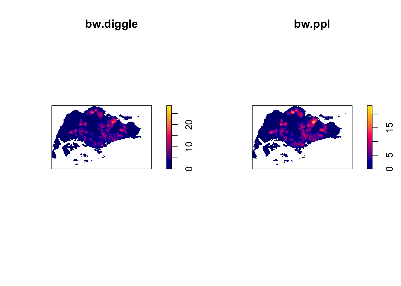
# Different kernel methods
par(mfrow=c(2,2))
plot(density(childcareSG_ppp.km,
sigma=bw.ppl,
edge=TRUE,
kernel="gaussian"),
main="Gaussian")
plot(density(childcareSG_ppp.km,
sigma=bw.ppl,
edge=TRUE,
kernel="epanechnikov"),
main="Epanechnikov")
plot(density(childcareSG_ppp.km,
sigma=bw.ppl,
edge=TRUE,
kernel="quartic"),
main="Quartic")
plot(density(childcareSG_ppp.km,
sigma=bw.ppl,
edge=TRUE,
kernel="disc"),
main="Disc")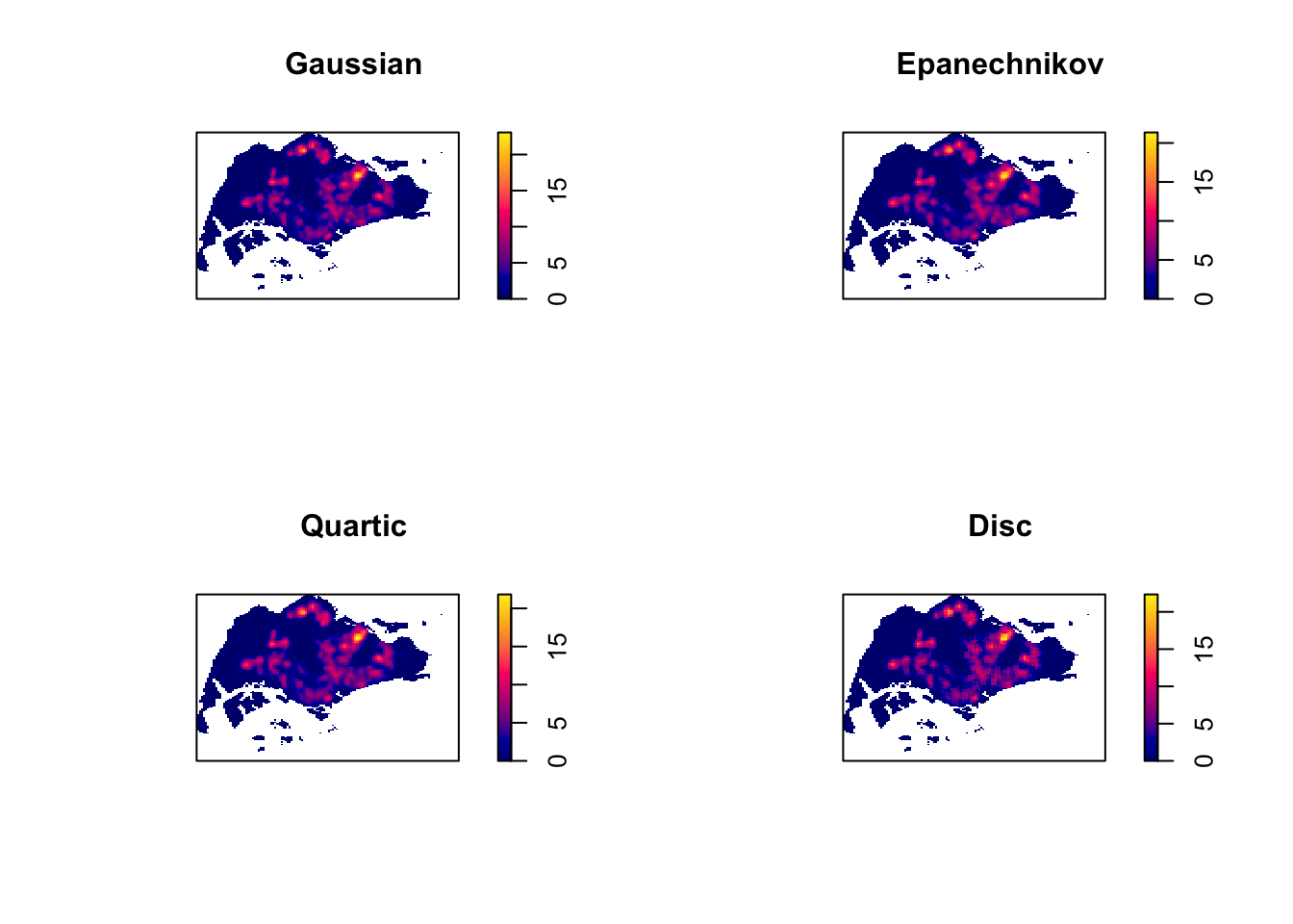
Fixed & Adaptive KDE
# Compute KDE with bw of 600m (sigma=0.6)
kde_childcareSG_600 <- density(childcareSG_ppp.km, sigma=0.6, edge=TRUE, kernel="gaussian")
plot(kde_childcareSG_600)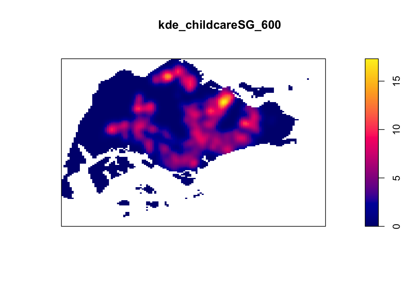
# KDE with adaptive bandwith
kde_childcareSG_adaptive <- adaptive.density(childcareSG_ppp.km, method="kernel")
plot(kde_childcareSG_adaptive)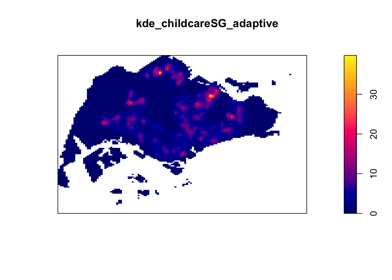
# Compared fixed vs adaptive
par(mfrow=c(1,2))
plot(kde_childcareSG.bw, main = "Fixed bandwidth")
plot(kde_childcareSG_adaptive, main = "Adaptive bandwidth")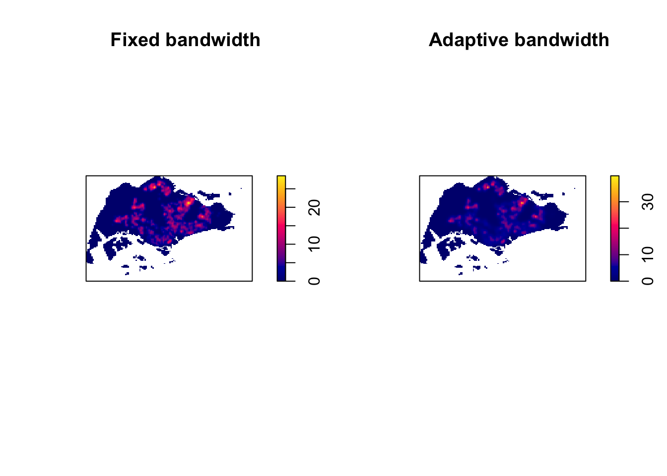
# KDE output into grid
gridded_kde_childcareSG_bw <- as.SpatialGridDataFrame.im(kde_childcareSG.bw)
spplot(gridded_kde_childcareSG_bw)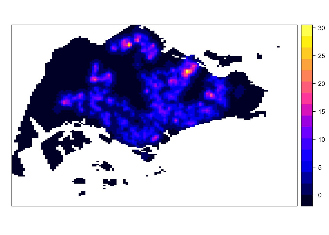
# grid to raster
kde_childcareSG_bw_raster <- raster(gridded_kde_childcareSG_bw)kde_childcareSG_bw_rasterclass : RasterLayer
dimensions : 128, 128, 16384 (nrow, ncol, ncell)
resolution : 0.4170614, 0.2647348 (x, y)
extent : 2.663926, 56.04779, 16.35798, 50.24403 (xmin, xmax, ymin, ymax)
crs : NA
source : memory
names : v
values : -1.005814e-14, 28.51831 (min, max)# include crs info into raster
projection(kde_childcareSG_bw_raster) <- CRS("+init=EPSG:3414")
kde_childcareSG_bw_rasterclass : RasterLayer
dimensions : 128, 128, 16384 (nrow, ncol, ncell)
resolution : 0.4170614, 0.2647348 (x, y)
extent : 2.663926, 56.04779, 16.35798, 50.24403 (xmin, xmax, ymin, ymax)
crs : +init=EPSG:3414
source : memory
names : v
values : -1.005814e-14, 28.51831 (min, max)# visualise output
tm_shape(kde_childcareSG_bw_raster) +
tm_raster("v") +
tm_layout(legend.position = c("right", "bottom"), frame = FALSE)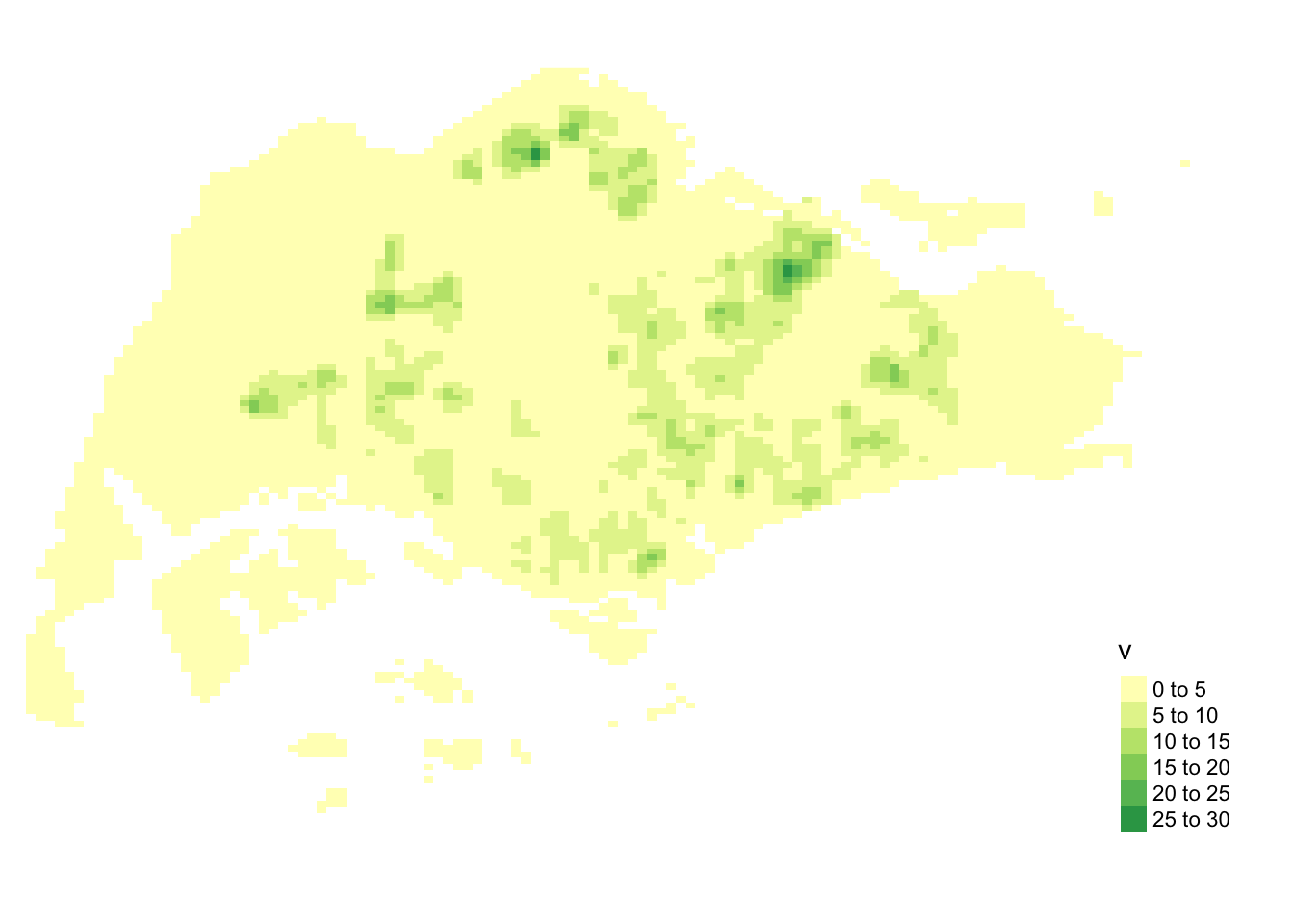
Comparing spatial point patterns using KDE
# Extract areas for analysis
pg = mpsz[mpsz@data$PLN_AREA_N == "PUNGGOL",]
tm = mpsz[mpsz@data$PLN_AREA_N == "TAMPINES",]
ck = mpsz[mpsz@data$PLN_AREA_N == "CHOA CHU KANG",]
jw = mpsz[mpsz@data$PLN_AREA_N == "JURONG WEST",]# plot
par(mfrow=c(2,2))
plot(pg, main = "Ponggol")
plot(tm, main = "Tampines")
plot(ck, main = "Choa Chu Kang")
plot(jw, main = "Jurong West")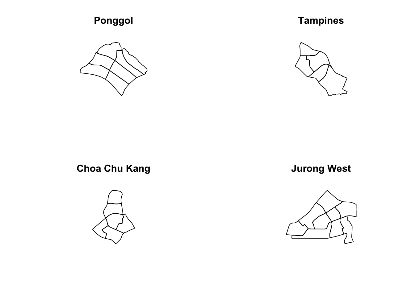
# convert to sp
pg_sp = as(pg, "SpatialPolygons")
tm_sp = as(tm, "SpatialPolygons")
ck_sp = as(ck, "SpatialPolygons")
jw_sp = as(jw, "SpatialPolygons")# convert to owin
pg_owin = as(pg_sp, "owin")
tm_owin = as(tm_sp, "owin")
ck_owin = as(ck_sp, "owin")
jw_owin = as(jw_sp, "owin")# extract childcare in regions
childcare_pg_ppp = childcare_ppp_jit[pg_owin]
childcare_tm_ppp = childcare_ppp_jit[tm_owin]
childcare_ck_ppp = childcare_ppp_jit[ck_owin]
childcare_jw_ppp = childcare_ppp_jit[jw_owin]# rescale to transform unit of measurement
childcare_pg_ppp.km = rescale(childcare_pg_ppp, 1000, "km")
childcare_tm_ppp.km = rescale(childcare_tm_ppp, 1000, "km")
childcare_ck_ppp.km = rescale(childcare_ck_ppp, 1000, "km")
childcare_jw_ppp.km = rescale(childcare_jw_ppp, 1000, "km")# Plot
par(mfrow=c(2,2))
plot(childcare_pg_ppp.km, main="Punggol")
plot(childcare_tm_ppp.km, main="Tampines")
plot(childcare_ck_ppp.km, main="Choa Chu Kang")
plot(childcare_jw_ppp.km, main="Jurong West")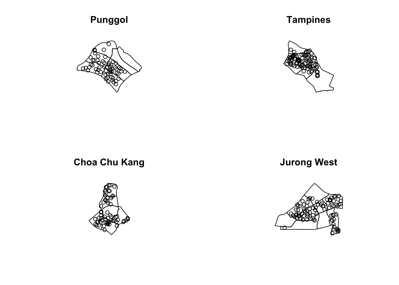
# computer KDE
par(mfrow=c(2,2))
plot(density(childcare_pg_ppp.km,
sigma=bw.diggle,
edge=TRUE,
kernel="gaussian"),
main="Punggol")
plot(density(childcare_tm_ppp.km,
sigma=bw.diggle,
edge=TRUE,
kernel="gaussian"),
main="Tempines")
plot(density(childcare_ck_ppp.km,
sigma=bw.diggle,
edge=TRUE,
kernel="gaussian"),
main="Choa Chu Kang")
plot(density(childcare_jw_ppp.km,
sigma=bw.diggle,
edge=TRUE,
kernel="gaussian"),
main="JUrong West")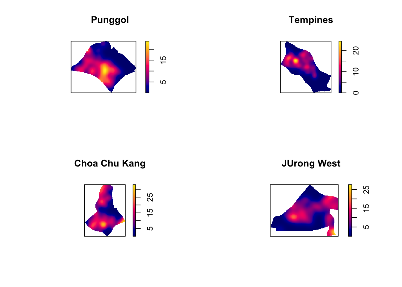
# compute fixed bandwith KDE
par(mfrow=c(2,2))
plot(density(childcare_ck_ppp.km,
sigma=0.25,
edge=TRUE,
kernel="gaussian"),
main="Chou Chu Kang")
plot(density(childcare_jw_ppp.km,
sigma=0.25,
edge=TRUE,
kernel="gaussian"),
main="JUrong West")
plot(density(childcare_pg_ppp.km,
sigma=0.25,
edge=TRUE,
kernel="gaussian"),
main="Punggol")
plot(density(childcare_tm_ppp.km,
sigma=0.25,
edge=TRUE,
kernel="gaussian"),
main="Tampines")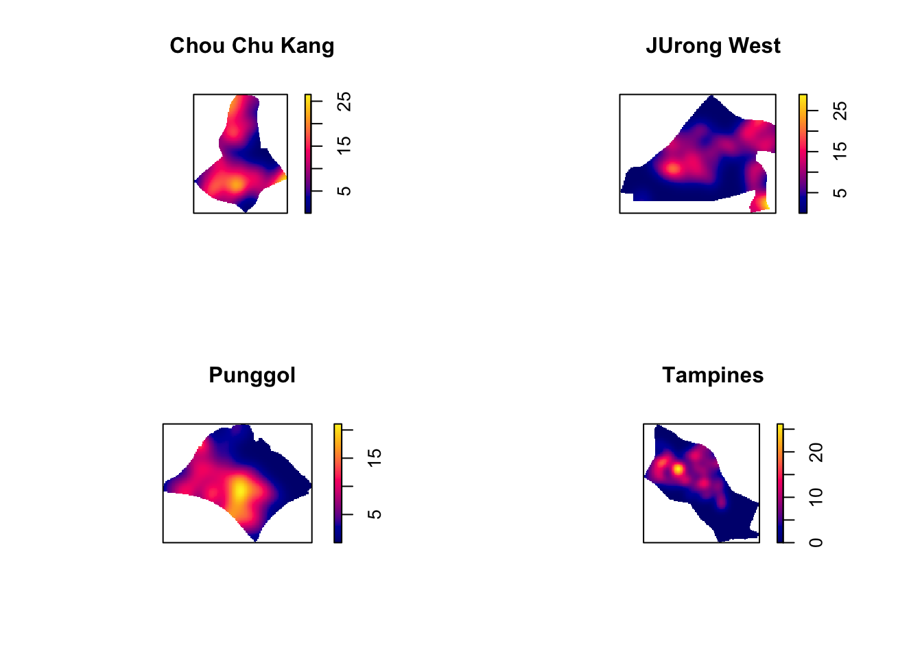
Nearest Neighbour Analysis
# Clark-Evans test of aggregation
clarkevans.test(childcareSG_ppp,
correction="none",
clipregion="sg_owin",
alternative=c("clustered"),
nsim=99)
Clark-Evans test
No edge correction
Monte Carlo test based on 99 simulations of CSR with fixed n
data: childcareSG_ppp
R = 0.54756, p-value = 0.01
alternative hypothesis: clustered (R < 1)# C-E test for CCK
clarkevans.test(childcare_ck_ppp,
correction="none",
clipregion=NULL,
alternative=c("two.sided"),
nsim=999)
Clark-Evans test
No edge correction
Monte Carlo test based on 999 simulations of CSR with fixed n
data: childcare_ck_ppp
R = 0.92672, p-value = 0.09
alternative hypothesis: two-sided# C-E test for Tamp
clarkevans.test(childcare_tm_ppp,
correction="none",
clipregion=NULL,
alternative=c("two.sided"),
nsim=999)
Clark-Evans test
No edge correction
Monte Carlo test based on 999 simulations of CSR with fixed n
data: childcare_tm_ppp
R = 0.79627, p-value = 0.002
alternative hypothesis: two-sidedSecond-Order Spatial Point Pattern Analysis
G Function
# Compute G-function using Gest()
G_CK = Gest(childcare_ck_ppp, correction = "border")
plot(G_CK, xlim=c(0,500))
# Monte Carlo test with G-function
G_CK.csr <- envelope(childcare_ck_ppp, Gest, nsim = 999)Generating 999 simulations of CSR ...
1, 2, 3, ......10.........20.........30.........40.........50.........60........
.70.........80.........90.........100.........110.........120.........130......
...140.........150.........160.........170.........180.........190.........200....
.....210.........220.........230.........240.........250.........260.........270..
.......280.........290.........300.........310.........320.........330.........340
.........350.........360.........370.........380.........390.........400........
.410.........420.........430.........440.........450.........460.........470......
...480.........490.........500.........510.........520.........530.........540....
.....550.........560.........570.........580.........590.........600.........610..
.......620.........630.........640.........650.........660.........670.........680
.........690.........700.........710.........720.........730.........740........
.750.........760.........770.........780.........790.........800.........810......
...820.........830.........840.........850.........860.........870.........880....
.....890.........900.........910.........920.........930.........940.........950..
.......960.........970.........980.........990........ 999.
Done.plot(G_CK.csr)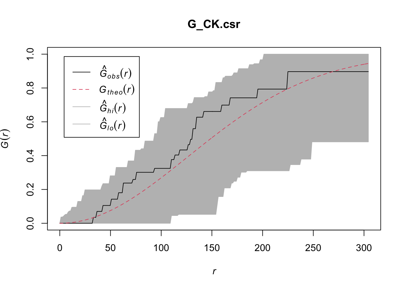
# Compute G-func for Tamp
G_tm = Gest(childcare_tm_ppp, correction = "best")
plot(G_tm)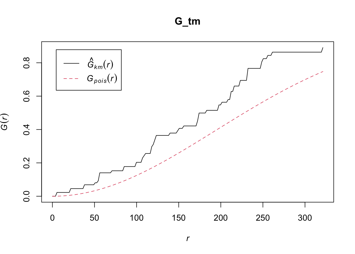
# Monte-Carole Test: Hypo test for random distribution in Tamp (H0=rand, H1=not rand)
G_tm.csr <- envelope(childcare_tm_ppp, Gest, correction = "all", nsim = 999)Generating 999 simulations of CSR ...
1, 2, 3, ......10.........20.........30.........40.........50.........60........
.70.........80.........90.........100.........110.........120.........130......
...140.........150.........160.........170.........180.........190.........200....
.....210.........220.........230.........240.........250.........260.........270..
.......280.........290.........300.........310.........320.........330.........340
.........350.........360.........370.........380.........390.........400........
.410.........420.........430.........440.........450.........460.........470......
...480.........490.........500.........510.........520.........530.........540....
.....550.........560.........570.........580.........590.........600.........610..
.......620.........630.........640.........650.........660.........670.........680
.........690.........700.........710.........720.........730.........740........
.750.........760.........770.........780.........790.........800.........810......
...820.........830.........840.........850.........860.........870.........880....
.....890.........900.........910.........920.........930.........940.........950..
.......960.........970.........980.........990........ 999.
Done.plot(G_tm.csr)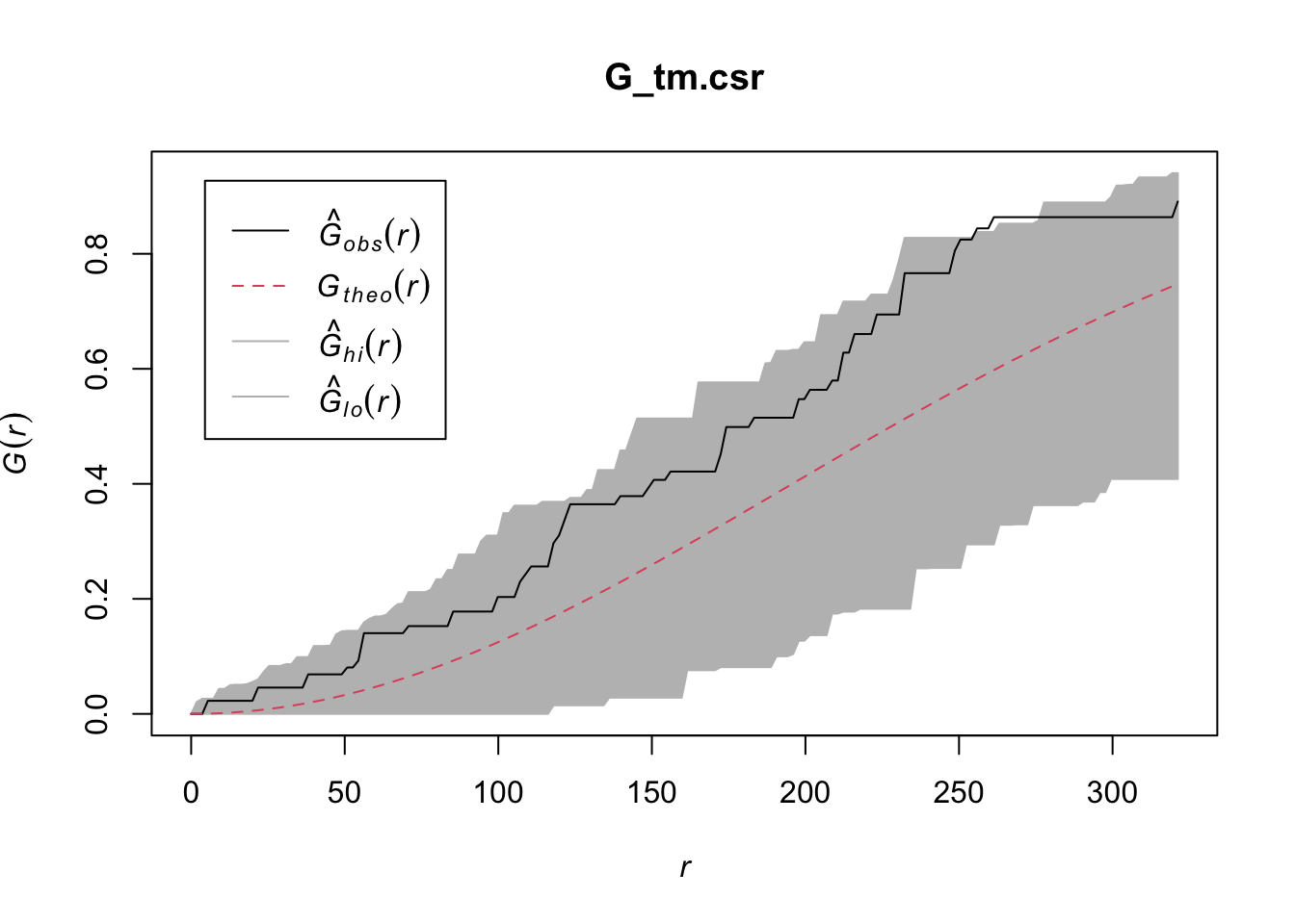
F Function
# Compute F-func on CCK
F_CK = Fest(childcare_ck_ppp)
plot(F_CK)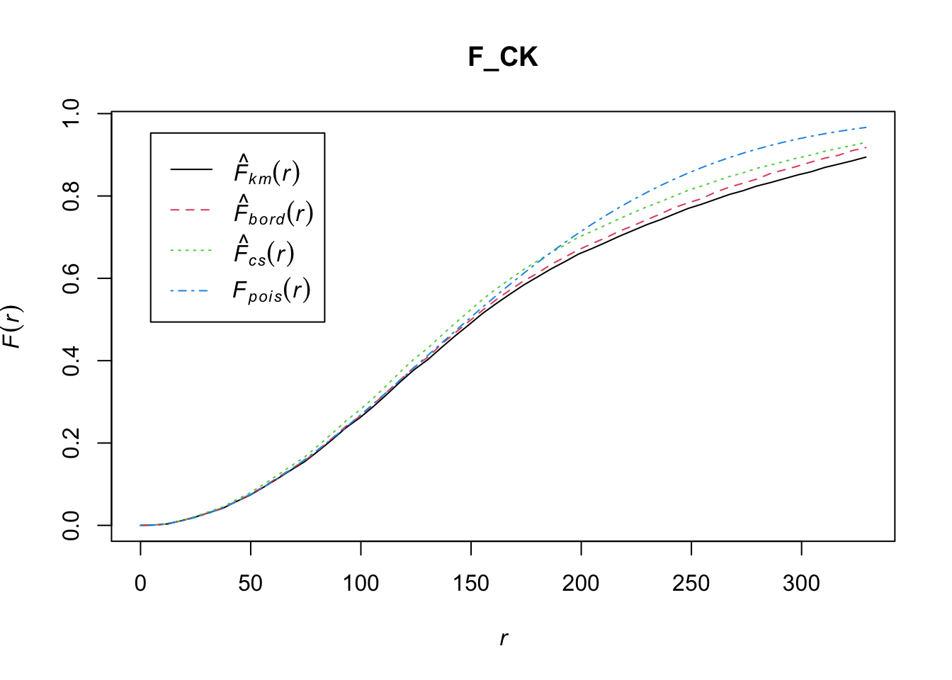
# Monte-Carole Test: Hypo testing for randomness (H0=rand, H1=not rand)
F_CK.csr <- envelope(childcare_ck_ppp, Fest, nsim = 999)Generating 999 simulations of CSR ...
1, 2, 3, ......10.........20.........30.........40.........50.........60........
.70.........80.........90.........100.........110.........120.........130......
...140.........150.........160.........170.........180.........190.........200....
.....210.........220.........230.........240.........250.........260.........270..
.......280.........290.........300.........310.........320.........330.........340
.........350.........360.........370.........380.........390.........400........
.410.........420.........430.........440.........450.........460.........470......
...480.........490.........500.........510.........520.........530.........540....
.....550.........560.........570.........580.........590.........600.........610..
.......620.........630.........640.........650.........660.........670.........680
.........690.........700.........710.........720.........730.........740........
.750.........760.........770.........780.........790.........800.........810......
...820.........830.........840.........850.........860.........870.........880....
.....890.........900.........910.........920.........930.........940.........950..
.......960.........970.........980.........990........ 999.
Done.# Plot results => lies within envelope, so insufficient evidence to reject null hypo, therefore is random
plot(F_CK.csr)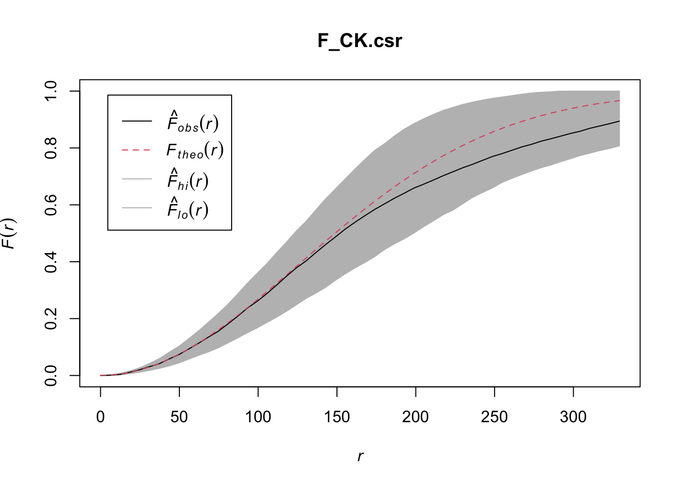
# Compute F func for tamp
F_tm = Fest(childcare_tm_ppp, correction = "best")
plot(F_tm)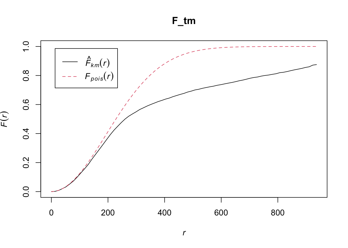
# Monte Carlo test for tamp
F_tm.csr <- envelope(childcare_tm_ppp, Fest, correction = "all", nsim = 999)Generating 999 simulations of CSR ...
1, 2, 3, ......10.........20.........30.........40.........50.........60........
.70.........80.........90.........100.........110.........120.........130......
...140.........150.........160.........170.........180.........190.........200....
.....210.........220.........230.........240.........250.........260.........270..
.......280.........290.........300.........310.........320.........330.........340
.........350.........360.........370.........380.........390.........400........
.410.........420.........430.........440.........450.........460.........470......
...480.........490.........500.........510.........520.........530.........540....
.....550.........560.........570.........580.........590.........600.........610..
.......620.........630.........640.........650.........660.........670.........680
.........690.........700.........710.........720.........730.........740........
.750.........760.........770.........780.........790.........800.........810......
...820.........830.........840.........850.........860.........870.........880....
.....890.........900.........910.........920.........930.........940.........950..
.......960.........970.........980.........990........ 999.
Done.plot(F_tm.csr)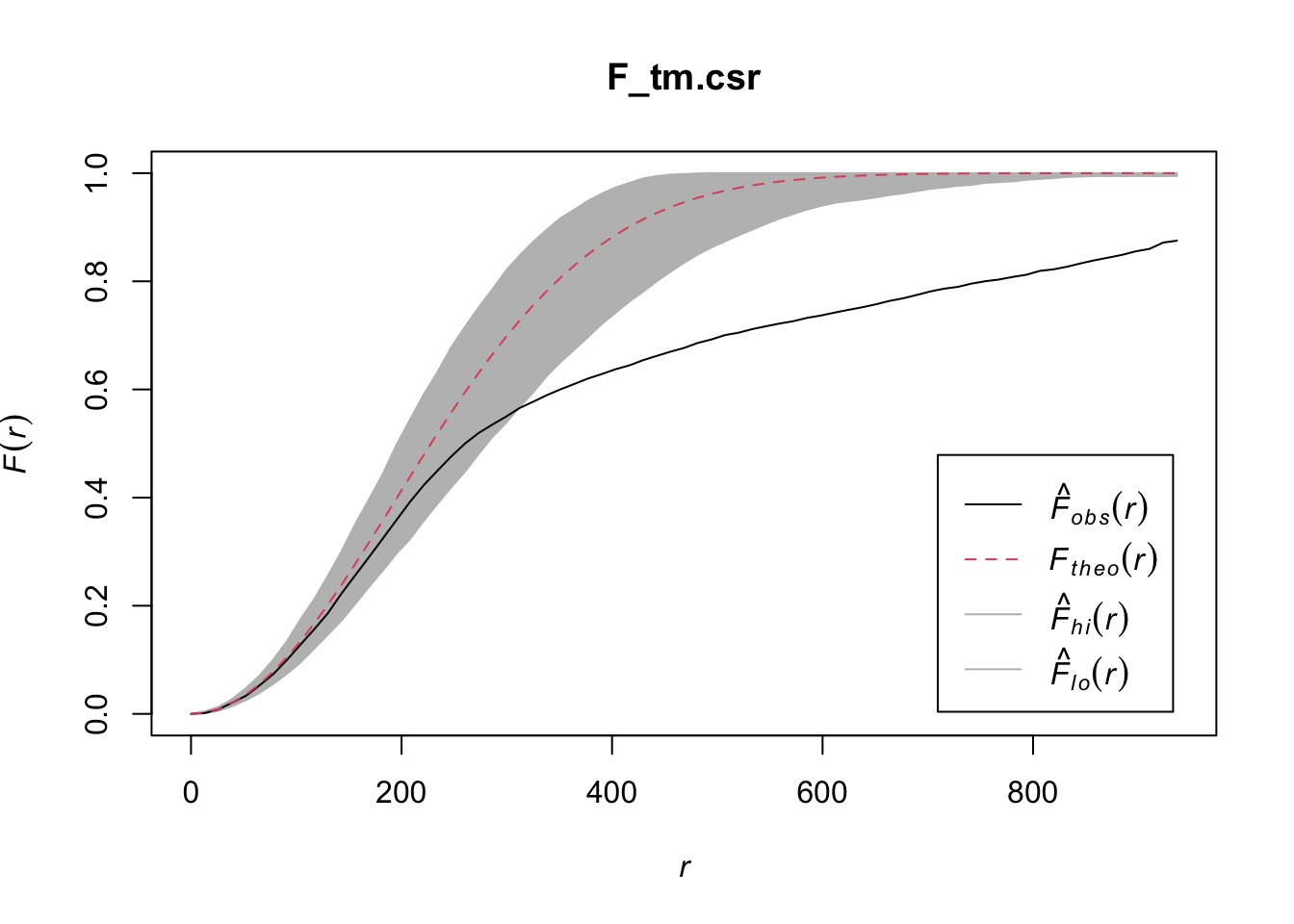
K Function
# Calc k func for cck
K_ck = Kest(childcare_ck_ppp, correction = "Ripley")
plot(K_ck, . -r ~ r, ylab= "K(d)-r", xlab = "d(m)")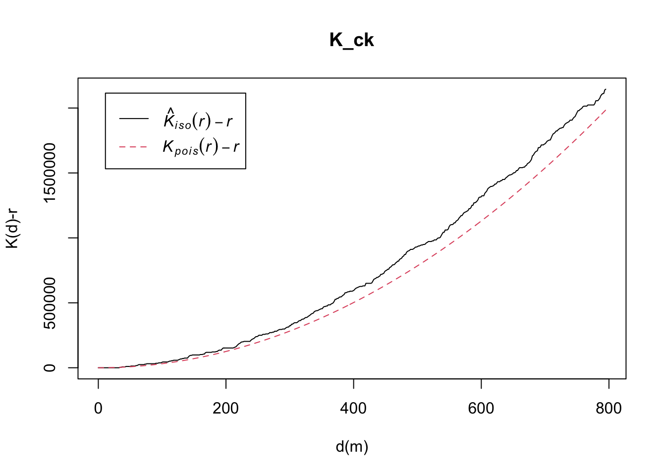
# Monte Carlo test for cck
K_ck.csr <- envelope(childcare_ck_ppp, Kest, nsim = 99, rank = 1, glocal=TRUE)Generating 99 simulations of CSR ...
1, 2, 3, 4, 5, 6, 7, 8, 9, 10, 11, 12, 13, 14, 15, 16, 17, 18, 19, 20, 21, 22, 23, 24, 25, 26, 27, 28, 29, 30, 31, 32, 33, 34, 35, 36, 37, 38, 39, 40,
41, 42, 43, 44, 45, 46, 47, 48, 49, 50, 51, 52, 53, 54, 55, 56, 57, 58, 59, 60, 61, 62, 63, 64, 65, 66, 67, 68, 69, 70, 71, 72, 73, 74, 75, 76, 77, 78, 79, 80,
81, 82, 83, 84, 85, 86, 87, 88, 89, 90, 91, 92, 93, 94, 95, 96, 97, 98, 99.
Done.plot(K_ck.csr, . - r ~ r, xlab="d", ylab="K(d)-r")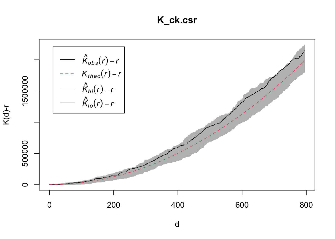
# K func for tamp
K_tm = Kest(childcare_tm_ppp, correction = "Ripley")
plot(K_tm, . -r ~ r,
ylab= "K(d)-r", xlab = "d(m)",
xlim=c(0,1000))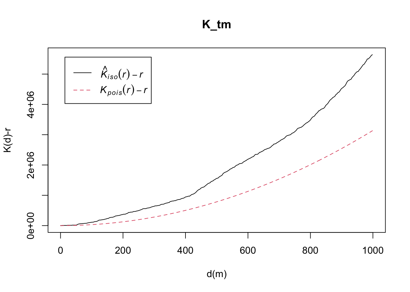
K_tm.csr <- envelope(childcare_tm_ppp, Kest, nsim = 99, rank = 1, glocal=TRUE)Generating 99 simulations of CSR ...
1, 2, 3, 4, 5, 6, 7, 8, 9, 10, 11, 12, 13, 14, 15, 16, 17, 18, 19, 20, 21, 22, 23, 24, 25, 26, 27, 28, 29, 30, 31, 32, 33, 34, 35, 36, 37, 38, 39, 40,
41, 42, 43, 44, 45, 46, 47, 48, 49, 50, 51, 52, 53, 54, 55, 56, 57, 58, 59, 60, 61, 62, 63, 64, 65, 66, 67, 68, 69, 70, 71, 72, 73, 74, 75, 76, 77, 78, 79, 80,
81, 82, 83, 84, 85, 86, 87, 88, 89, 90, 91, 92, 93, 94, 95, 96, 97, 98, 99.
Done.plot(K_tm.csr, . - r ~ r,
xlab="d", ylab="K(d)-r", xlim=c(0,500))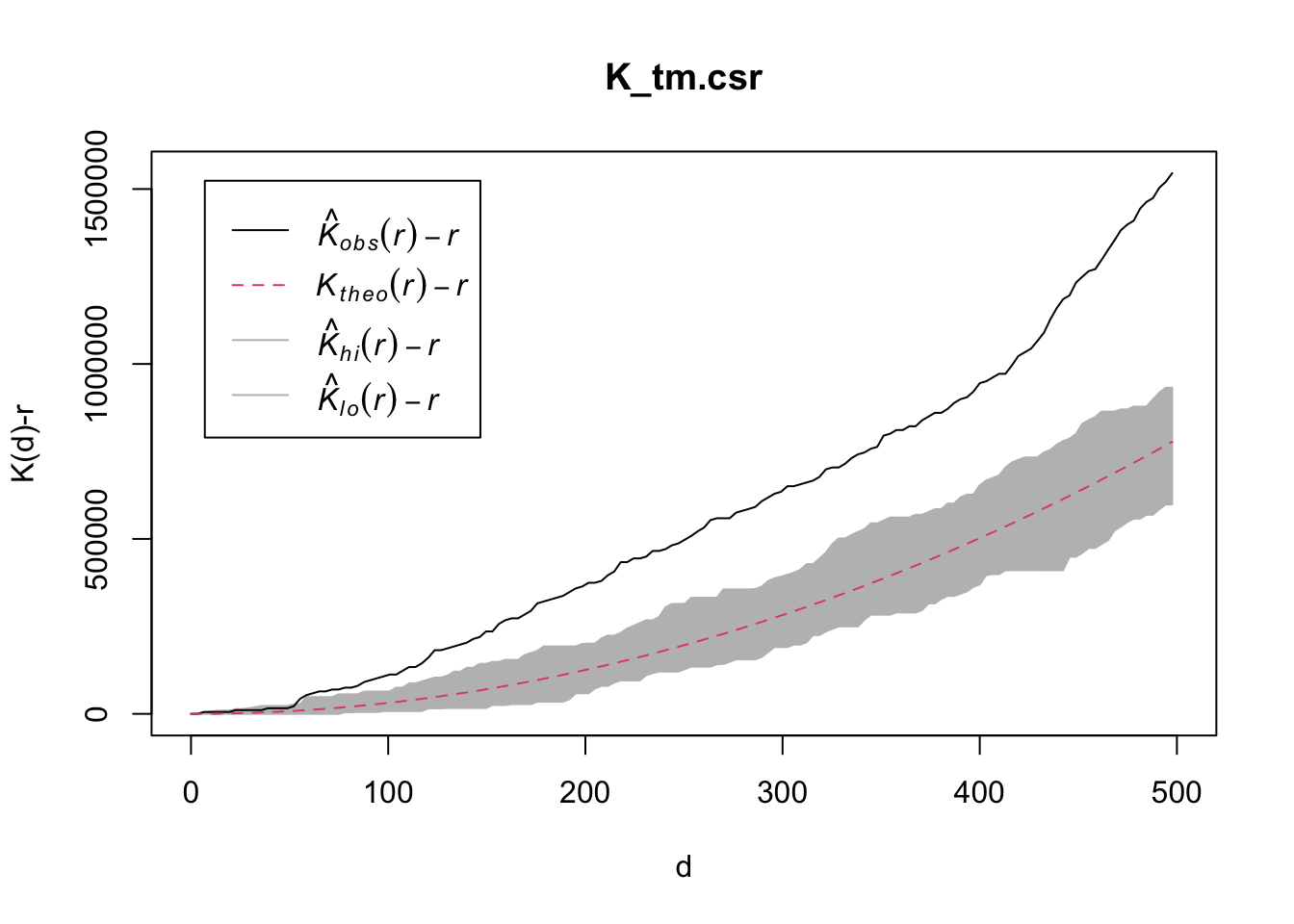
L Function
# L func for cck
L_ck = Lest(childcare_ck_ppp, correction = "Ripley")
plot(L_ck, . -r ~ r,
ylab= "L(d)-r", xlab = "d(m)")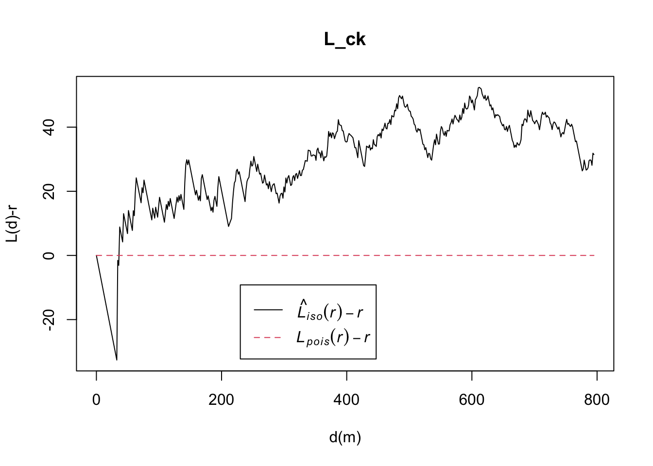
L_ck.csr <- envelope(childcare_ck_ppp, Lest, nsim = 99, rank = 1, glocal=TRUE)Generating 99 simulations of CSR ...
1, 2, 3, 4, 5, 6, 7, 8, 9, 10, 11, 12, 13, 14, 15, 16, 17, 18, 19, 20, 21, 22, 23, 24, 25, 26, 27, 28, 29, 30, 31, 32, 33, 34, 35, 36, 37, 38, 39, 40,
41, 42, 43, 44, 45, 46, 47, 48, 49, 50, 51, 52, 53, 54, 55, 56, 57, 58, 59, 60, 61, 62, 63, 64, 65, 66, 67, 68, 69, 70, 71, 72, 73, 74, 75, 76, 77, 78, 79, 80,
81, 82, 83, 84, 85, 86, 87, 88, 89, 90, 91, 92, 93, 94, 95, 96, 97, 98, 99.
Done.plot(L_ck.csr, . - r ~ r, xlab="d", ylab="L(d)-r")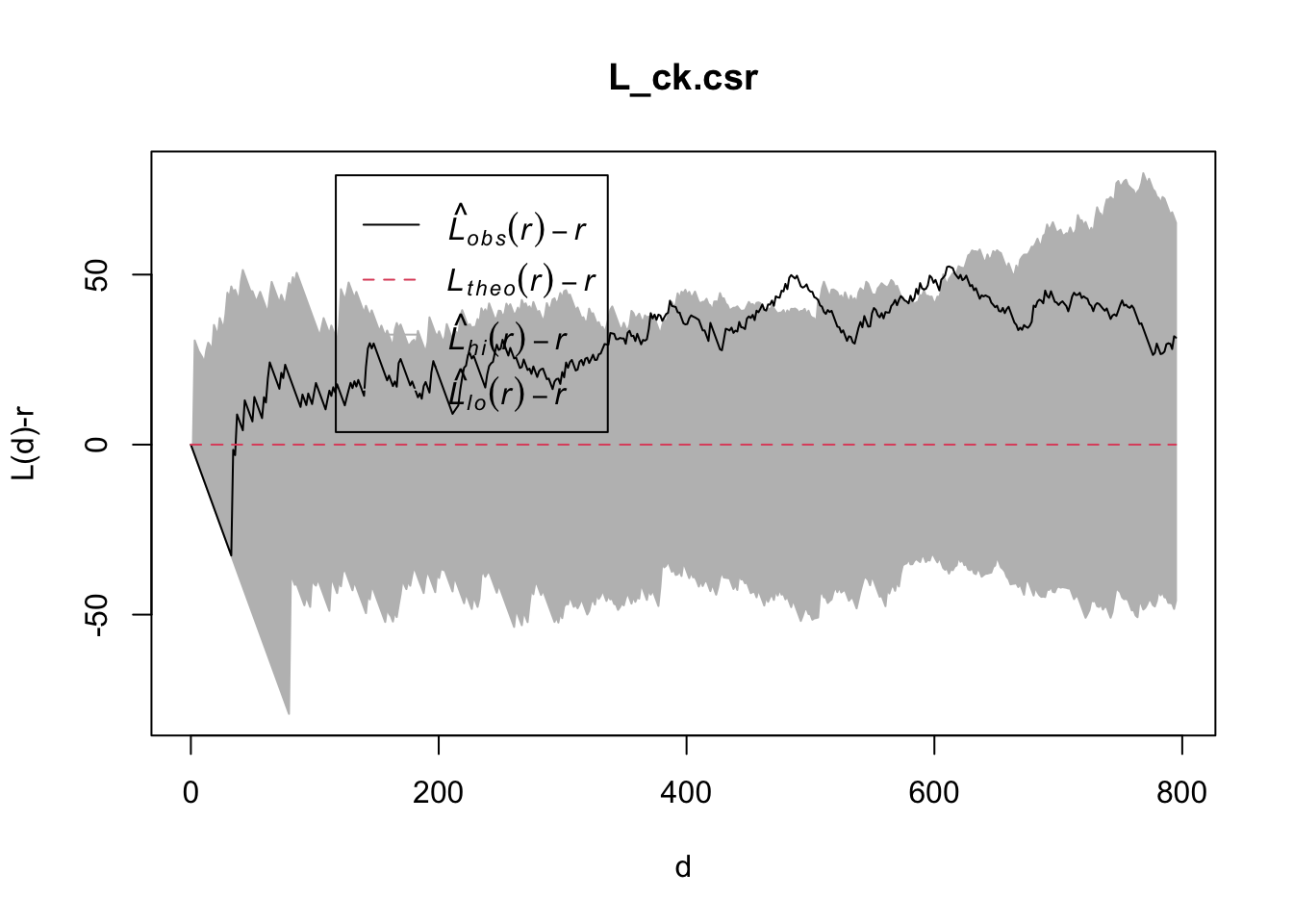
# L func for cck
L_tm = Lest(childcare_tm_ppp, correction = "Ripley")
plot(L_tm, . -r ~ r,
ylab= "L(d)-r", xlab = "d(m)",
xlim=c(0,1000))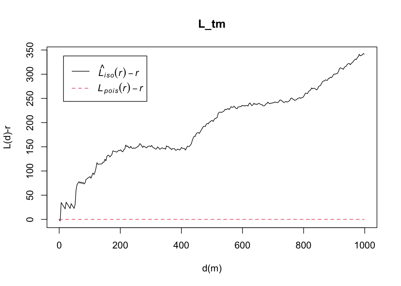
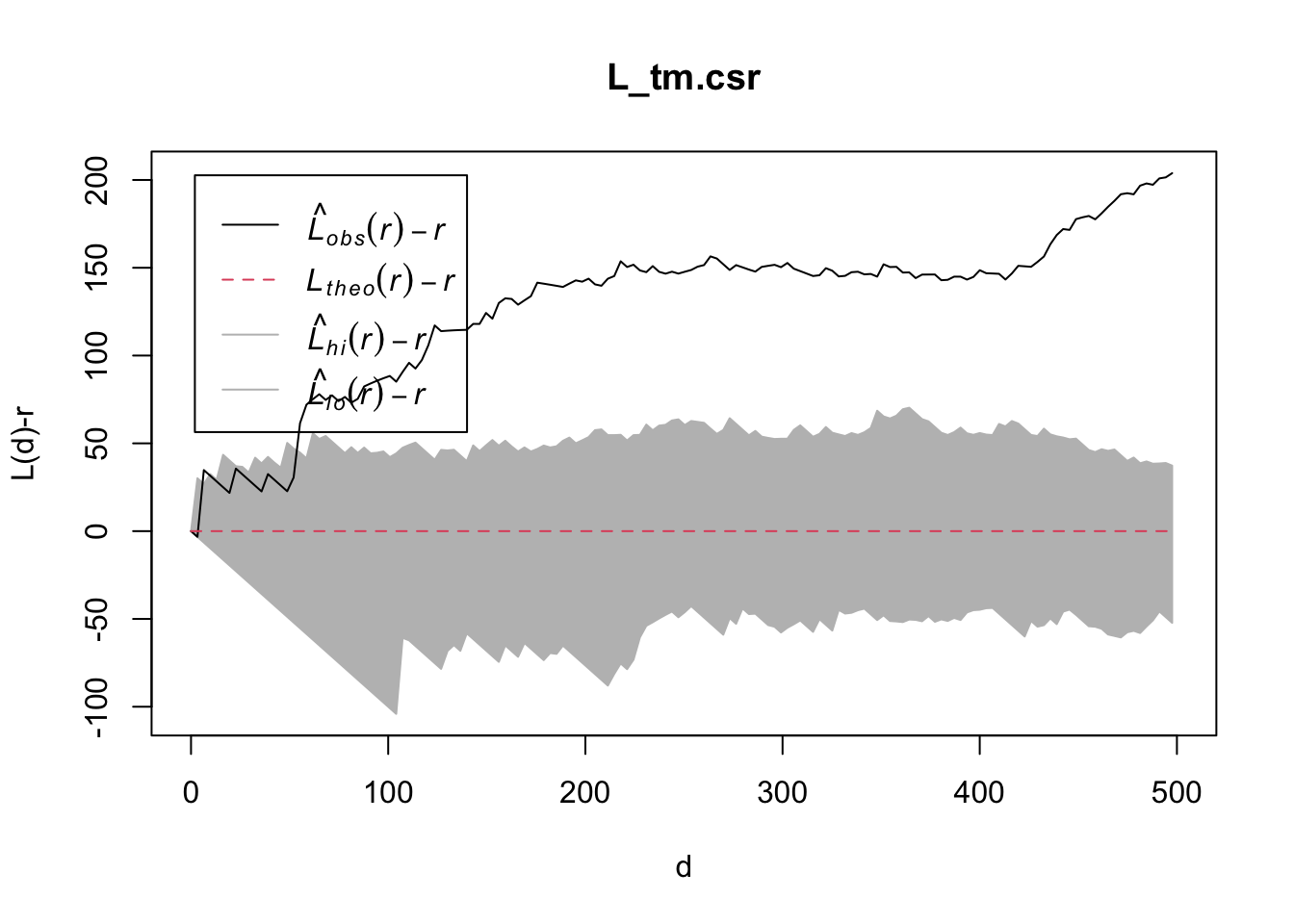
L_tm.csr <- envelope(childcare_tm_ppp, Lest, nsim = 99, rank = 1, glocal=TRUE)Generating 99 simulations of CSR ...
1, 2, 3, 4, 5, 6, 7, 8, 9, 10, 11, 12, 13, 14, 15, 16, 17, 18, 19, 20, 21, 22, 23, 24, 25, 26, 27, 28, 29, 30, 31, 32, 33, 34, 35, 36, 37, 38, 39, 40,
41, 42, 43, 44, 45, 46, 47, 48, 49, 50, 51, 52, 53, 54, 55, 56, 57, 58, 59, 60, 61, 62, 63, 64, 65, 66, 67, 68, 69, 70, 71, 72, 73, 74, 75, 76, 77, 78, 79, 80,
81, 82, 83, 84, 85, 86, 87, 88, 89, 90, 91, 92, 93, 94, 95, 96, 97, 98, 99.
Done.plot(L_tm.csr, . - r ~ r,
xlab="d", ylab="L(d)-r", xlim=c(0,500))