pacman::p_load(sf, sfdep, tmap, tidyverse, plotly)In-Class Exercise 7: Global and Local Measures of Spatial Association
Imports
Import data
# Import
hunan <- st_read(dsn = "data/geospatial",
                 layer = "Hunan")
Reading layer `Hunan' from data source
`/Users/michelle/Desktop/IS415/shelle-mim/IS415-GAA/In-class_Exercise/Wk7/data/geospatial'
using driver `ESRI Shapefile'
Simple feature collection with 88 features and 7 fields
Geometry type: POLYGON
Dimension: XY
Bounding box: xmin: 108.7831 ymin: 24.6342 xmax: 114.2544 ymax: 30.12812
Geodetic CRS: WGS 84hunan2012 <- read_csv("data/aspatial/Hunan_2012.csv")
# Join the data
hunan_GDPPC <- left_join(hunan, hunan2012) %>% # left one must be the geospatial
select(1:4, 7, 15)# Visualise the data
tm_shape(hunan_GDPPC)+
tm_fill("GDPPC",
style = "quantile",
palette = "RdPu",
title = "Dependency ratio") +
tm_layout(main.title = "Distribution of GDP per capita by district, Hunan Province",
main.title.position = "center",
main.title.size = 1,
legend.outside = TRUE,
frame = TRUE) +
tm_borders(alpha = 0.5) +
tm_grid(alpha =0.2) +
tm_compass(type="8star", size = 2) +
tm_scale_bar()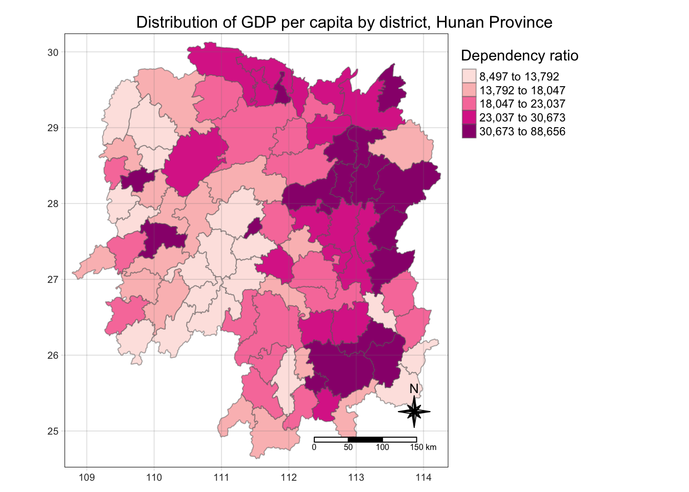
Global Measures of Spatial Association
Derive weight metrics
wm_q <- hunan_GDPPC %>%
  mutate(nb = st_contiguity(geometry),
         wt = st_weights(nb,
                         style = "W"),
         .before = 1)

wm_q # is not a typical data struct, has lists within. saved within a data table
Simple feature collection with 88 features and 8 fields
Geometry type: POLYGON
Dimension: XY
Bounding box: xmin: 108.7831 ymin: 24.6342 xmax: 114.2544 ymax: 30.12812
Geodetic CRS: WGS 84
First 10 features:
nb
1 2, 3, 4, 57, 85
2 1, 57, 58, 78, 85
3 1, 4, 5, 85
4 1, 3, 5, 6
5 3, 4, 6, 85
6 4, 5, 69, 75, 85
7 67, 71, 74, 84
8 9, 46, 47, 56, 78, 80, 86
9 8, 66, 68, 78, 84, 86
10 16, 17, 19, 20, 22, 70, 72, 73
wt
1 0.2, 0.2, 0.2, 0.2, 0.2
2 0.2, 0.2, 0.2, 0.2, 0.2
3 0.25, 0.25, 0.25, 0.25
4 0.25, 0.25, 0.25, 0.25
5 0.25, 0.25, 0.25, 0.25
6 0.2, 0.2, 0.2, 0.2, 0.2
7 0.25, 0.25, 0.25, 0.25
8 0.1428571, 0.1428571, 0.1428571, 0.1428571, 0.1428571, 0.1428571, 0.1428571
9 0.1666667, 0.1666667, 0.1666667, 0.1666667, 0.1666667, 0.1666667
10 0.125, 0.125, 0.125, 0.125, 0.125, 0.125, 0.125, 0.125
NAME_2 ID_3 NAME_3 ENGTYPE_3 County GDPPC
1 Changde 21098 Anxiang County Anxiang 23667
2 Changde 21100 Hanshou County Hanshou 20981
3 Changde 21101 Jinshi County City Jinshi 34592
4 Changde 21102 Li County Li 24473
5 Changde 21103 Linli County Linli 25554
6 Changde 21104 Shimen County Shimen 27137
7 Changsha 21109 Liuyang County City Liuyang 63118
8 Changsha 21110 Ningxiang County Ningxiang 62202
9 Changsha 21111 Wangcheng County Wangcheng 70666
10 Chenzhou 21112 Anren County Anren 12761
geometry
1 POLYGON ((112.0625 29.75523...
2 POLYGON ((112.2288 29.11684...
3 POLYGON ((111.8927 29.6013,...
4 POLYGON ((111.3731 29.94649...
5 POLYGON ((111.6324 29.76288...
6 POLYGON ((110.8825 30.11675...
7 POLYGON ((113.9905 28.5682,...
8 POLYGON ((112.7181 28.38299...
9 POLYGON ((112.7914 28.52688...
10 POLYGON ((113.1757 26.82734...Computing Global Moran’I
moranI <- global_moran(wm_q$GDPPC, #need to specify which vectors bcos its a diff data struct
                       wm_q$nb,
                       wm_q$wt)
Perform Global Moran’I test
# Usually dont just conpute moranI by itself, do the global test
global_moran_test(wm_q$GDPPC, # need to specify which vectors bcos its a diff data struct
                  wm_q$nb,
                  wm_q$wt)
    Moran I test under randomisation

data:  x
weights: listw

Moran I statistic standard deviate = 4.7351, p-value = 1.095e-06
alternative hypothesis: greater
sample estimates:
Moran I statistic       Expectation          Variance
      0.300749970      -0.011494253       0.004348351
Perform Global Moran’I permutation test
set.seed(42069) # put in seperate code chunk so is global# Perform Monte Carlo simulation
global_moran_perm(wm_q$GDPPC, # need to specify which vectors bcos its a diff data struct
wm_q$nb,
wm_q$wt,
nsim = 99)
    Monte-Carlo simulation of Moran I

data:  x
weights: listw
number of simulations + 1: 100

statistic = 0.30075, observed rank = 100, p-value < 2.2e-16
alternative hypothesis: two.sided
Computing local Moran’s I
lisa <- wm_q %>%
  mutate(local_moran = local_moran(GDPPC, nb, wt, nsim = 99),
    .before = 1) %>%
  unnest(local_moran)

lisa # will automatically give you the low-low, high-low, high-high, do not need to manually translate it
Simple feature collection with 88 features and 20 fields
Geometry type: POLYGON
Dimension: XY
Bounding box: xmin: 108.7831 ymin: 24.6342 xmax: 114.2544 ymax: 30.12812
Geodetic CRS: WGS 84
# A tibble: 88 × 21
ii eii var_ii z_ii p_ii p_ii_…¹ p_fol…² skewn…³ kurto…⁴
<dbl> <dbl> <dbl> <dbl> <dbl> <dbl> <dbl> <dbl> <dbl>
1 -0.00147 -0.000102 0.000610 -0.0554 9.56e-1 0.78 0.39 -0.935 0.478
2 0.0259 0.00777 0.00796 0.203 8.39e-1 0.98 0.49 -0.601 -0.102
3 -0.0120 0.0256 0.140 -0.100 9.20e-1 0.84 0.42 0.858 -0.0960
4 0.00102 -0.000341 0.00000485 0.620 5.36e-1 0.5 0.25 1.15 0.807
5 0.0148 0.00160 0.00137 0.356 7.22e-1 0.66 0.33 0.748 0.379
6 -0.0388 -0.0196 0.00691 -0.231 8.17e-1 0.98 0.49 0.989 1.04
7 3.37 0.124 2.23 2.17 2.97e-2 0.12 0.06 1.42 2.07
8 1.56 -0.240 0.645 2.24 2.50e-2 0.06 0.03 0.508 0.147
9 4.42 -0.0736 1.39 3.82 1.34e-4 0.02 0.01 0.555 -0.396
10 -0.399 -0.00709 0.0749 -1.43 1.52e-1 0.26 0.13 -0.392 -0.765
# … with 78 more rows, 12 more variables: mean <fct>, median <fct>,
# pysal <fct>, nb <nb>, wt <list>, NAME_2 <chr>, ID_3 <int>, NAME_3 <chr>,
# ENGTYPE_3 <chr>, County <chr>, GDPPC <dbl>, geometry <POLYGON [°]>, and
# abbreviated variable names ¹p_ii_sim, ²p_folded_sim, ³skewness, ⁴kurtosis# will generally use the mean or the pysal for the resultVisualising local Moran’s I
# Plot moran'i
tmap_mode("plot")
tm_shape(lisa) +
  tm_fill("ii") +
  tm_borders(alpha = 0.5)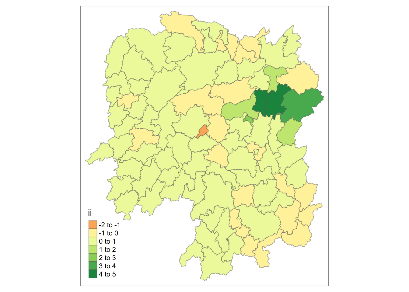
# Plot p value
# p_ii_sim from the one with many simulations
tm_shape(lisa) +
  tm_fill("p_ii_sim") +
  tm_borders(alpha = 0.5)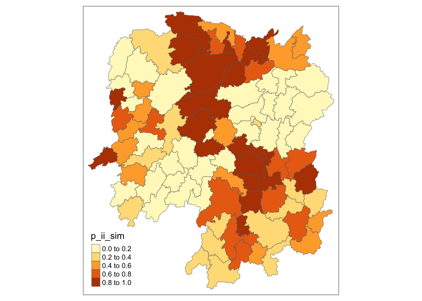
lisa_sig <- lisa %>%
  filter(p_ii_sim < 0.05)

# plot the significant low-low, low-high, high-low and high-high
tm_shape(lisa) +
  tm_polygons() +
  tm_borders(alpha = 0.5) +
  tm_shape(lisa_sig) +
  tm_fill("mean") +
  tm_borders(alpha = 0.4)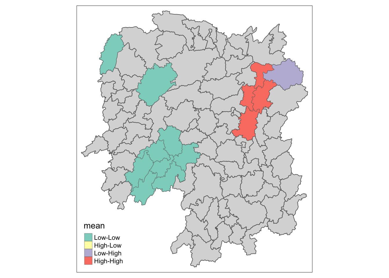
Hot Spot & Cold Spot Area Analysis (HCSA)
Computing local Gi* statistics
wm_idw <- hunan_GDPPC %>%
  mutate(nb = st_contiguity(geometry),
         wts = st_inverse_distance(nb, geometry,
                                   scale = 1,
                                   alpha = 1),
         .before = 1)
HCSA <- wm_idw %>%
mutate(local_Gi = local_gstar_perm(GDPPC, nb, wt, nsim=99),
.before = 1) %>%
unnest(local_Gi)
HCSASimple feature collection with 88 features and 16 fields
Geometry type: POLYGON
Dimension: XY
Bounding box: xmin: 108.7831 ymin: 24.6342 xmax: 114.2544 ymax: 30.12812
Geodetic CRS: WGS 84
# A tibble: 88 × 17
gi_star e_gi var_gi p_value p_sim p_fold…¹ skewn…² kurto…³ nb wts
<dbl> <dbl> <dbl> <dbl> <dbl> <dbl> <dbl> <dbl> <nb> <lis>
1 -0.0578 0.0117 0.00000946 9.54e- 1 0.92 0.46 0.573 -0.638 <int> <dbl>
2 -0.456 0.0117 0.00000740 6.48e- 1 0.78 0.39 0.426 -0.472 <int> <dbl>
3 0.369 0.0110 0.0000109 7.12e- 1 0.64 0.32 0.967 0.436 <int> <dbl>
4 0.412 0.0113 0.0000103 6.80e- 1 0.58 0.29 0.664 -0.350 <int> <dbl>
5 0.181 0.0119 0.0000109 8.56e- 1 0.88 0.44 0.490 -0.201 <int> <dbl>
6 -0.377 0.0114 0.00000778 7.06e- 1 0.86 0.43 0.422 -0.656 <int> <dbl>
7 3.70 0.0113 0.00000860 2.18e- 4 0.02 0.01 0.906 0.354 <int> <dbl>
8 2.64 0.0108 0.00000607 8.20e- 3 0.06 0.03 0.914 0.390 <int> <dbl>
9 6.24 0.0106 0.00000388 4.44e-10 0.02 0.01 0.228 -0.749 <int> <dbl>
10 1.15 0.0112 0.00000539 2.48e- 1 0.32 0.16 0.573 -0.275 <int> <dbl>
# … with 78 more rows, 7 more variables: NAME_2 <chr>, ID_3 <int>,
# NAME_3 <chr>, ENGTYPE_3 <chr>, County <chr>, GDPPC <dbl>,
# geometry <POLYGON [°]>, and abbreviated variable names ¹p_folded_sim,
# ²skewness, ³kurtosisVisualising Gi*
tmap_mode("view")
tm_shape(HCSA) +
  tm_fill("gi_star") +
  tm_borders(alpha = 0.5) +
  tm_view(set.zoom.limits = c(6, 8))
Visualising p-value of HCSA
# plot significant values
tmap_mode("plot")

tm_shape(HCSA) +
  tm_fill("p_sim") +
  tm_borders(alpha = 0.5)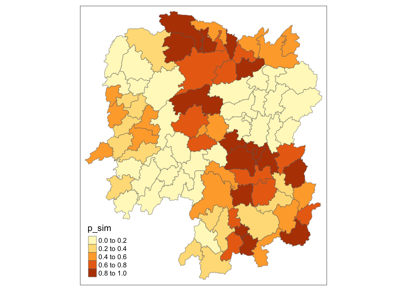
Visualising hot spot & cold spot areas
HCSA_sig <- HCSA  %>%
  filter(p_sim < 0.05)
tmap_mode("plot")
tm_shape(HCSA) +
  tm_polygons() +
  tm_borders(alpha = 0.5) +
tm_shape(HCSA_sig) +
  tm_fill("gi_star") +
  tm_borders(alpha = 0.4)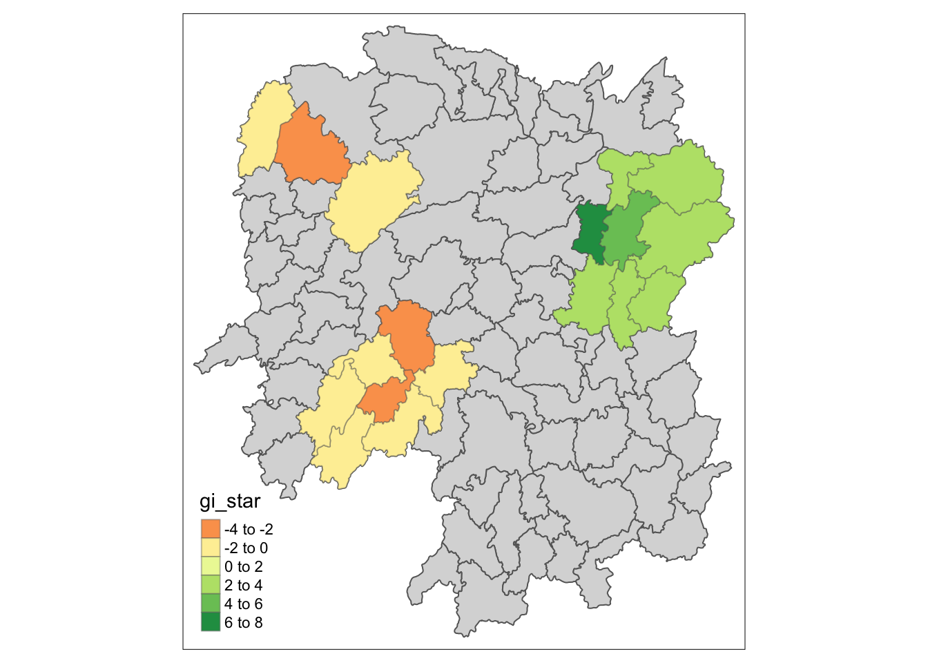
Emerging Hot Spot Analysis
Import Data
GDPPC <- read_csv("data/aspatial/Hunan_GDPPC.csv")Creating a Time Series Cube
GDPPC_st = spacetime(GDPPC, hunan, .loc_col = "County", .time_col = "Year")is_spacetime_cube(GDPPC_st)[1] TRUEComputing Gi*
Deriving spatial weights
GDPPC_nb <- GDPPC_st %>%
  activate("geometry") %>%
  mutate(
    nb = include_self(st_contiguity(geometry)),
    wt = st_weights(nb)
  ) %>%
  set_nbs("nb") %>%
set_wts("wt")head(GDPPC_nb)# A tibble: 6 × 5
Year County GDPPC nb wt
<dbl> <chr> <dbl> <list> <list>
1 2005 Anxiang 8184 <int [6]> <dbl [6]>
2 2005 Hanshou 6560 <int [6]> <dbl [6]>
3 2005 Jinshi 9956 <int [5]> <dbl [5]>
4 2005 Li 8394 <int [5]> <dbl [5]>
5 2005 Linli 8850 <int [5]> <dbl [5]>
6 2005 Shimen 9244 <int [6]> <dbl [6]>Compute Gi*
gi_stars <- GDPPC_nb %>%
  group_by(Year) %>%
  mutate(gi_star = local_gstar_perm(
    GDPPC, nb, wt)) %>%
  tidyr::unnest(gi_star)
Mann-Kendall Test
cbg <- gi_stars %>%
  ungroup() %>%
  filter(County == "Changsha") %>%
  select(County, Year, gi_star)
# Plot
ggplot(data = cbg,
aes(x = Year,
y = gi_star)) +
geom_line() +
theme_light()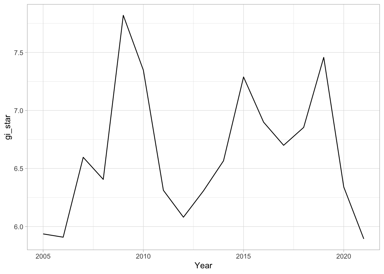
# Interative plot
p <- ggplot(data = cbg,
       aes(x = Year,
           y = gi_star)) +
  geom_line() +
  theme_light()

ggplotly(p)
# get p-value (sl)
cbg %>%
summarise(mk = list(
unclass(
Kendall::MannKendall(gi_star)))) %>%
tidyr::unnest_wider(mk)# A tibble: 1 × 5
tau sl S D varS
<dbl> <dbl> <dbl> <dbl> <dbl>
1 0.118 0.537 16 136. 589.# Replicate for each location using group_by()
ehsa <- gi_stars %>%
group_by(County) %>%
summarise(mk = list(
unclass(
Kendall::MannKendall(gi_star)))) %>%
tidyr::unnest_wider(mk)Arrange to show sig values
emerging <- ehsa %>%
  arrange(sl, abs(tau)) %>%
  slice(1:5)
Performing Emerging Hotspot
ehsa <- emerging_hotspot_analysis(
  x = GDPPC_st,
  .var = "GDPPC",
  k = 1,
  nsim = 99
)
Visualising distribution of EHSA classes
ggplot(data = ehsa,
       aes(x = classification)) +
  ggplot2::geom_bar()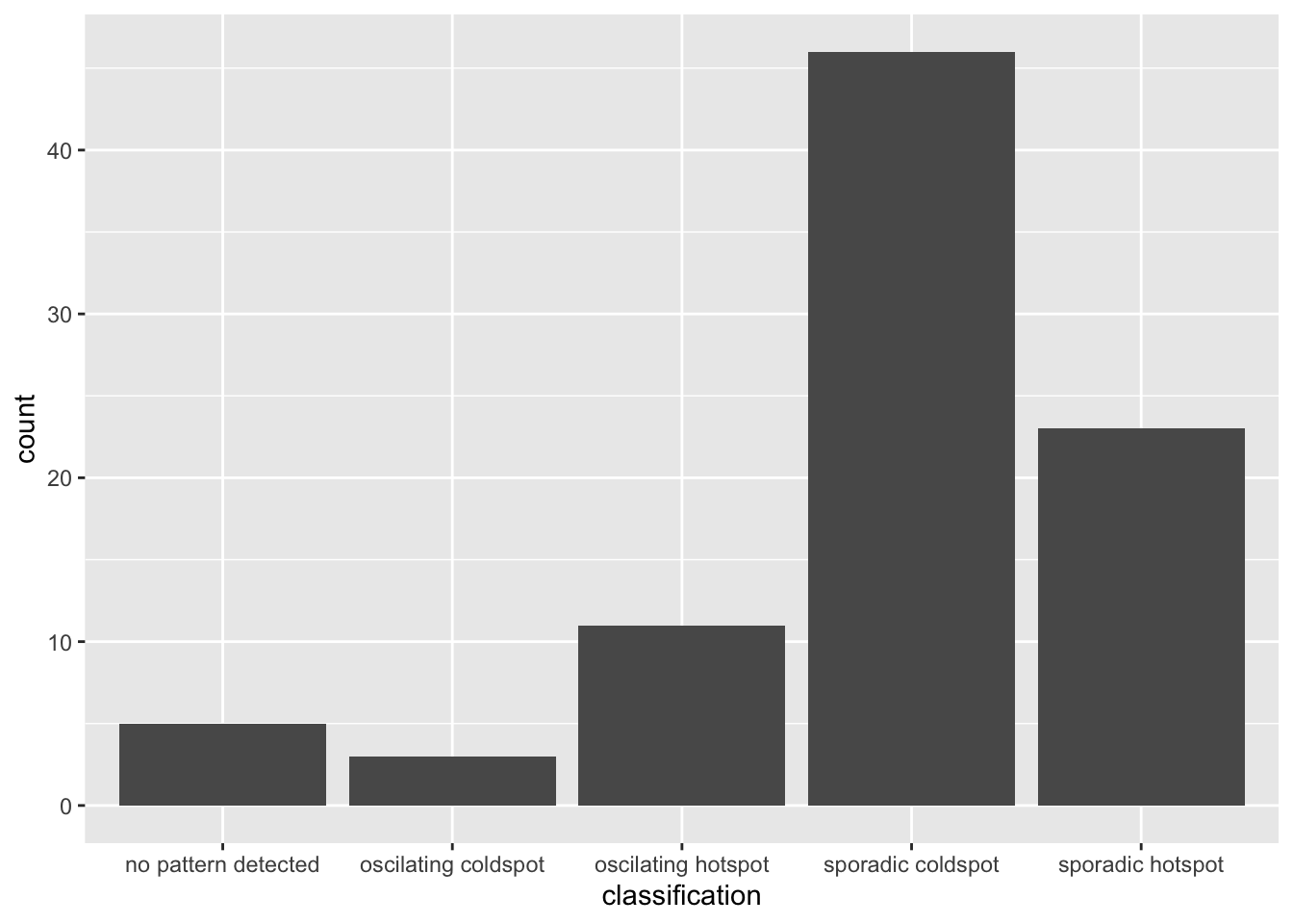
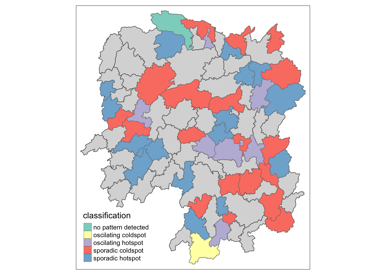
Visualising EHSA
# join ehsa to hunan data
hunan_ehsa <- hunan %>%
  left_join(ehsa, by = c("County" = "location"))
# plot
ehsa_sig <- hunan_ehsa %>%
filter(p_value < 0.05)
tmap_mode("plot")
tm_shape(hunan_ehsa) +
tm_polygons() +
tm_borders(alpha = 0.5) +
tm_shape(ehsa_sig) +
tm_fill("classification") +
tm_borders(alpha = 0.4)