pacman::p_load(sf, sfdep, tmap, tidyverse, plotly, readxl)Take-Home Exercise 2: Spatio-temporal Analysis of COVID-19 Vaccination Trends in DKI Jakarta
Introduction
Background & Objective
In this exercise, we will be investigating Covid-19 vaccination trends in Jakarta, Indonesia. In order to do this, we will be using Geospatial data of the layout of Jakarta, as well as Aspatial data in the form of daily vaccination data in order to calculate and analyse the vaccination rates in Jakarta.
Defining the Study Area
For this study, we will confine the study area between July 2021 and June 2022. This is to best capture the vaccination rates during the time period where vaccinations were fire widely available as well as Covid rapidly spreading.
In this assignment, we will be selecting the data from the last day of each month in order to summarise the data for that particular month.
Import Packages
For this exercise, we will be using the following packages:
sf for importing, managing, and processing geospatial data
sfdep for performing geospatial data wrangling and Hotspot & Coldspot Analysis
tidyverse for performing data science tasks such as importing, wrangling and visualising data
tmap which provides functions for plotting cartographic quality static point patterns maps or interactive maps
plotly for plotting graphs
and readxl for loading data from .xlsx files
Import the Data
Now, let us import our data into our project.
Import Geospatial Data
jakarta_boundaries <- st_read(dsn="data/geospatial",
                      layer="BATAS_DESA_DESEMBER_2019_DUKCAPIL_DKI_JAKARTA")
Reading layer `BATAS_DESA_DESEMBER_2019_DUKCAPIL_DKI_JAKARTA' from data source
`/Users/michelle/Desktop/IS415/shelle-mim/IS415-GAA/Take-home_Exercise/TH2/data/geospatial'
using driver `ESRI Shapefile'
Simple feature collection with 269 features and 161 fields
Geometry type: MULTIPOLYGON
Dimension: XY
Bounding box: xmin: 106.3831 ymin: -6.370815 xmax: 106.9728 ymax: -5.184322
Geodetic CRS: WGS 84Import Aspatial Data
# Load Excel Files
jul2021_raw <- read_xlsx("data/aspatial/Data Vaksinasi Berbasis Kelurahan (31 Juli 2021).xlsx")
aug2021_raw <- read_xlsx("data/aspatial/Data Vaksinasi Berbasis Kelurahan (31 Agustus 2021).xlsx")
sep2021_raw <- read_xlsx("data/aspatial/Data Vaksinasi Berbasis Kelurahan (30 September 2021).xlsx")
oct2021_raw <- read_xlsx("data/aspatial/Data Vaksinasi Berbasis Kelurahan (31 Oktober 2021).xlsx")
nov2021_raw <- read_xlsx("data/aspatial/Data Vaksinasi Berbasis Kelurahan (30 November 2021).xlsx")
dec2021_raw <- read_xlsx("data/aspatial/Data Vaksinasi Berbasis Kelurahan (31 Desember 2021).xlsx")
jan2022_raw <- read_xlsx("data/aspatial/Data Vaksinasi Berbasis Kelurahan (31 Januari 2022).xlsx")
feb2022_raw <- read_xlsx("data/aspatial/Data Vaksinasi Berbasis Kelurahan (27 Februari 2022).xlsx")
mar2022_raw <- read_xlsx("data/aspatial/Data Vaksinasi Berbasis Kelurahan (31 Maret 2022).xlsx")
apr2022_raw <- read_xlsx("data/aspatial/Data Vaksinasi Berbasis Kelurahan (30 April 2022).xlsx")
may2022_raw <- read_xlsx("data/aspatial/Data Vaksinasi Berbasis Kelurahan (31 Mei 2022).xlsx")
jun2022_raw <- read_xlsx("data/aspatial/Data Vaksinasi Berbasis Kelurahan (30 Juni 2022).xlsx")
# Add the month as a column before joining
jul2021 <- jul2021_raw %>% add_column(Date = "31 Jul 2021")
aug2021 <- aug2021_raw %>% add_column(Date = "31 Aug 2021")
sep2021 <- sep2021_raw %>% add_column(Date = "30 Sep 2021")
oct2021 <- oct2021_raw %>% add_column(Date = "31 Oct 2021")
nov2021 <- nov2021_raw %>% add_column(Date = "30 Nov 2021")
dec2021 <- dec2021_raw %>% add_column(Date = "31 Dec 2021")
jan2022 <- jan2022_raw %>% add_column(Date = "31 Jan 2022")
feb2022 <- feb2022_raw %>% add_column(Date = "27 Feb 2022")
mar2022 <- mar2022_raw %>% add_column(Date = "31 Mar 2022")
apr2022 <- apr2022_raw %>% add_column(Date = "30 Apr 2022")
may2022 <- may2022_raw %>% add_column(Date = "31 May 2022")
jun2022 <- jun2022_raw %>% add_column(Date = "30 Jun 2022")vaccination_data_list <- list(jul2021, aug2021, sep2021, oct2021, nov2021, dec2021, jan2022, feb2022, mar2022, apr2022, may2022, jun2022)
combined_vaccination_data <- reduce(vaccination_data_list, bind_rows)vaccination_data_list[[1]]
# A tibble: 268 × 28
KODE KELURA…¹ WILAY…² KECAM…³ KELUR…⁴ SASARAN BELUM…⁵ JUMLA…⁶ JUMLA…⁷ TOTAL…⁸
<chr> <chr> <chr> <chr> <dbl> <dbl> <dbl> <dbl> <dbl>
1 <NA> <NA> <NA> TOTAL 8941211 4441501 4499710 1663218 6162928
2 3172051003 JAKART… PADEMA… ANCOL 23947 12333 11614 4181 15795
3 3173041007 JAKART… TAMBORA ANGKE 29381 13875 15506 4798 20304
4 3175041005 JAKART… KRAMAT… BALE K… 29074 18314 10760 3658 14418
5 3175031003 JAKART… JATINE… BALI M… 9752 5173 4579 2007 6586
6 3175101006 JAKART… CIPAYU… BAMBU … 26285 13775 12510 5206 17716
7 3174031002 JAKART… MAMPAN… BANGKA 21566 10443 11123 4010 15133
8 3175051002 JAKART… PASAR … BARU 23886 10063 13823 6118 19941
9 3175041004 JAKART… KRAMAT… BATU A… 47898 28848 19050 7261 26311
10 3171071002 JAKART… TANAH … BENDUN… 21494 9978 11516 4602 16118
# … with 258 more rows, 19 more variables: `LANSIA\r\nDOSIS 1` <dbl>,
# `LANSIA\r\nDOSIS 2` <dbl>, `LANSIA TOTAL \r\nVAKSIN DIBERIKAN` <dbl>,
# `PELAYAN PUBLIK\r\nDOSIS 1` <dbl>, `PELAYAN PUBLIK\r\nDOSIS 2` <dbl>,
# `PELAYAN PUBLIK TOTAL\r\nVAKSIN DIBERIKAN` <dbl>,
# `GOTONG ROYONG\r\nDOSIS 1` <dbl>, `GOTONG ROYONG\r\nDOSIS 2` <dbl>,
# `GOTONG ROYONG TOTAL\r\nVAKSIN DIBERIKAN` <dbl>,
# `TENAGA KESEHATAN\r\nDOSIS 1` <dbl>, `TENAGA KESEHATAN\r\nDOSIS 2` <dbl>, …
[[2]]
# A tibble: 268 × 28
KODE KELURA…¹ WILAY…² KECAM…³ KELUR…⁴ SASARAN BELUM…⁵ JUMLA…⁶ JUMLA…⁷ TOTAL…⁸
<chr> <chr> <chr> <chr> <dbl> <dbl> <dbl> <dbl> <dbl>
1 <NA> <NA> <NA> TOTAL 8941211 3277484 5663727 3412906 9076633
2 3172051003 JAKART… PADEMA… ANCOL 23947 9191 14756 8935 23691
3 3173041007 JAKART… TAMBORA ANGKE 29381 10400 18981 10470 29451
4 3175041005 JAKART… KRAMAT… BALE K… 29074 12510 16564 7766 24330
5 3175031003 JAKART… JATINE… BALI M… 9752 3704 6048 3671 9719
6 3175101006 JAKART… CIPAYU… BAMBU … 26285 9416 16869 10118 26987
7 3174031002 JAKART… MAMPAN… BANGKA 21566 8345 13221 8177 21398
8 3175051002 JAKART… PASAR … BARU 23886 7751 16135 11238 27373
9 3175041004 JAKART… KRAMAT… BATU A… 47898 19908 27990 15342 43332
10 3171071002 JAKART… TANAH … BENDUN… 21494 8033 13461 8671 22132
# … with 258 more rows, 19 more variables: `LANSIA\r\nDOSIS 1` <dbl>,
# `LANSIA\r\nDOSIS 2` <dbl>, `LANSIA TOTAL \r\nVAKSIN DIBERIKAN` <dbl>,
# `PELAYAN PUBLIK\r\nDOSIS 1` <dbl>, `PELAYAN PUBLIK\r\nDOSIS 2` <dbl>,
# `PELAYAN PUBLIK TOTAL\r\nVAKSIN DIBERIKAN` <dbl>,
# `GOTONG ROYONG\r\nDOSIS 1` <dbl>, `GOTONG ROYONG\r\nDOSIS 2` <dbl>,
# `GOTONG ROYONG TOTAL\r\nVAKSIN DIBERIKAN` <dbl>,
# `TENAGA KESEHATAN\r\nDOSIS 1` <dbl>, `TENAGA KESEHATAN\r\nDOSIS 2` <dbl>, …
[[3]]
# A tibble: 268 × 28
KODE KELURA…¹ WILAY…² KECAM…³ KELUR…⁴ SASARAN BELUM…⁵ JUMLA…⁶ JUMLA…⁷ TOTAL…⁸
<chr> <chr> <chr> <chr> <dbl> <dbl> <dbl> <dbl> <dbl>
1 <NA> <NA> <NA> TOTAL 8941211 2235772 6705439 5171697 1.19e7
2 3172051003 JAKART… PADEMA… ANCOL 23947 6688 17259 13376 3.06e4
3 3173041007 JAKART… TAMBORA ANGKE 29381 7581 21800 16438 3.82e4
4 3175041005 JAKART… KRAMAT… BALE K… 29074 8708 20366 14412 3.48e4
5 3175031003 JAKART… JATINE… BALI M… 9752 2517 7235 5660 1.29e4
6 3175101006 JAKART… CIPAYU… BAMBU … 26285 6252 20033 15380 3.54e4
7 3174031002 JAKART… MAMPAN… BANGKA 21566 5785 15781 12158 2.79e4
8 3175051002 JAKART… PASAR … BARU 23886 4899 18987 15536 3.45e4
9 3175041004 JAKART… KRAMAT… BATU A… 47898 14105 33793 24706 5.85e4
10 3171071002 JAKART… TANAH … BENDUN… 21494 5239 16255 12764 2.90e4
# … with 258 more rows, 19 more variables: `LANSIA\r\nDOSIS 1` <dbl>,
# `LANSIA\r\nDOSIS 2` <dbl>, `LANSIA TOTAL \r\nVAKSIN DIBERIKAN` <dbl>,
# `PELAYAN PUBLIK\r\nDOSIS 1` <dbl>, `PELAYAN PUBLIK\r\nDOSIS 2` <dbl>,
# `PELAYAN PUBLIK TOTAL\r\nVAKSIN DIBERIKAN` <dbl>,
# `GOTONG ROYONG\r\nDOSIS 1` <dbl>, `GOTONG ROYONG\r\nDOSIS 2` <dbl>,
# `GOTONG ROYONG TOTAL\r\nVAKSIN DIBERIKAN` <dbl>,
# `TENAGA KESEHATAN\r\nDOSIS 1` <dbl>, `TENAGA KESEHATAN\r\nDOSIS 2` <dbl>, …
[[4]]
# A tibble: 268 × 28
KODE KELURA…¹ WILAY…² KECAM…³ KELUR…⁴ SASARAN BELUM…⁵ JUMLA…⁶ JUMLA…⁷ TOTAL…⁸
<chr> <chr> <chr> <chr> <dbl> <dbl> <dbl> <dbl> <dbl>
1 <NA> <NA> <NA> TOTAL 8941211 1880524 7060687 5729001 1.28e7
2 3172051003 JAKART… PADEMA… ANCOL 23947 5991 17956 14504 3.25e4
3 3173041007 JAKART… TAMBORA ANGKE 29381 6557 22824 18185 4.10e4
4 3175041005 JAKART… KRAMAT… BALE K… 29074 7586 21488 16444 3.79e4
5 3175031003 JAKART… JATINE… BALI M… 9752 2125 7627 6277 1.39e4
6 3175101006 JAKART… CIPAYU… BAMBU … 26285 5014 21271 17291 3.86e4
7 3174031002 JAKART… MAMPAN… BANGKA 21566 4742 16824 13579 3.04e4
8 3175051002 JAKART… PASAR … BARU 23886 4089 19797 16697 3.65e4
9 3175041004 JAKART… KRAMAT… BATU A… 47898 12196 35702 27942 6.36e4
10 3171071002 JAKART… TANAH … BENDUN… 21494 4492 17002 14176 3.12e4
# … with 258 more rows, 19 more variables: `LANSIA\r\nDOSIS 1` <dbl>,
# `LANSIA\r\nDOSIS 2` <dbl>, `LANSIA TOTAL \r\nVAKSIN DIBERIKAN` <dbl>,
# `PELAYAN PUBLIK\r\nDOSIS 1` <dbl>, `PELAYAN PUBLIK\r\nDOSIS 2` <dbl>,
# `PELAYAN PUBLIK TOTAL\r\nVAKSIN DIBERIKAN` <dbl>,
# `GOTONG ROYONG\r\nDOSIS 1` <dbl>, `GOTONG ROYONG\r\nDOSIS 2` <dbl>,
# `GOTONG ROYONG TOTAL\r\nVAKSIN DIBERIKAN` <dbl>,
# `TENAGA KESEHATAN\r\nDOSIS 1` <dbl>, `TENAGA KESEHATAN\r\nDOSIS 2` <dbl>, …
[[5]]
# A tibble: 268 × 28
KODE KELURA…¹ WILAY…² KECAM…³ KELUR…⁴ SASARAN BELUM…⁵ JUMLA…⁶ JUMLA…⁷ TOTAL…⁸
<chr> <chr> <chr> <chr> <dbl> <dbl> <dbl> <dbl> <dbl>
1 <NA> <NA> <NA> TOTAL 8941211 1723821 7217390 6172636 1.34e7
2 3172051003 JAKART… PADEMA… ANCOL 23947 5527 18420 15466 3.39e4
3 3173041007 JAKART… TAMBORA ANGKE 29381 5986 23395 19404 4.28e4
4 3175041005 JAKART… KRAMAT… BALE K… 29074 6802 22272 18084 4.04e4
5 3175031003 JAKART… JATINE… BALI M… 9752 1920 7832 6773 1.46e4
6 3175101006 JAKART… CIPAYU… BAMBU … 26285 4612 21673 18694 4.04e4
7 3174031002 JAKART… MAMPAN… BANGKA 21566 4346 17220 14694 3.19e4
8 3175051002 JAKART… PASAR … BARU 23886 3776 20110 17781 3.79e4
9 3175041004 JAKART… KRAMAT… BATU A… 47898 10985 36913 30676 6.76e4
10 3171071002 JAKART… TANAH … BENDUN… 21494 4187 17307 15114 3.24e4
# … with 258 more rows, 19 more variables: `LANSIA\r\nDOSIS 1` <dbl>,
# `LANSIA\r\nDOSIS 2` <dbl>, `LANSIA TOTAL \r\nVAKSIN DIBERIKAN` <dbl>,
# `PELAYAN PUBLIK\r\nDOSIS 1` <dbl>, `PELAYAN PUBLIK\r\nDOSIS 2` <dbl>,
# `PELAYAN PUBLIK TOTAL\r\nVAKSIN DIBERIKAN` <dbl>,
# `GOTONG ROYONG\r\nDOSIS 1` <dbl>, `GOTONG ROYONG\r\nDOSIS 2` <dbl>,
# `GOTONG ROYONG TOTAL\r\nVAKSIN DIBERIKAN` <dbl>,
# `TENAGA KESEHATAN\r\nDOSIS 1` <dbl>, `TENAGA KESEHATAN\r\nDOSIS 2` <dbl>, …
[[6]]
# A tibble: 268 × 28
KODE KELURA…¹ WILAY…² KECAM…³ KELUR…⁴ SASARAN BELUM…⁵ JUMLA…⁶ JUMLA…⁷ TOTAL…⁸
<chr> <chr> <chr> <chr> <dbl> <dbl> <dbl> <dbl> <dbl>
1 <NA> <NA> <NA> TOTAL 8941211 1623736 7317475 6370175 1.37e7
2 3172051003 JAKART… PADEMA… ANCOL 23947 5062 18885 15996 3.49e4
3 3173041007 JAKART… TAMBORA ANGKE 29381 5626 23755 20026 4.38e4
4 3175041005 JAKART… KRAMAT… BALE K… 29074 6335 22739 18925 4.17e4
5 3175031003 JAKART… JATINE… BALI M… 9752 1782 7970 7003 1.50e4
6 3175101006 JAKART… CIPAYU… BAMBU … 26285 4373 21912 19400 4.13e4
7 3174031002 JAKART… MAMPAN… BANGKA 21566 4169 17397 15138 3.25e4
8 3175051002 JAKART… PASAR … BARU 23886 3579 20307 18239 3.85e4
9 3175041004 JAKART… KRAMAT… BATU A… 47898 10178 37720 32015 6.97e4
10 3171071002 JAKART… TANAH … BENDUN… 21494 3993 17501 15541 3.30e4
# … with 258 more rows, 19 more variables: `LANSIA\r\nDOSIS 1` <dbl>,
# `LANSIA\r\nDOSIS 2` <dbl>, `LANSIA TOTAL \r\nVAKSIN DIBERIKAN` <dbl>,
# `PELAYAN PUBLIK\r\nDOSIS 1` <dbl>, `PELAYAN PUBLIK\r\nDOSIS 2` <dbl>,
# `PELAYAN PUBLIK TOTAL\r\nVAKSIN DIBERIKAN` <dbl>,
# `GOTONG ROYONG\r\nDOSIS 1` <dbl>, `GOTONG ROYONG\r\nDOSIS 2` <dbl>,
# `GOTONG ROYONG TOTAL\r\nVAKSIN DIBERIKAN` <dbl>,
# `TENAGA KESEHATAN\r\nDOSIS 1` <dbl>, `TENAGA KESEHATAN\r\nDOSIS 2` <dbl>, …
[[7]]
# A tibble: 268 × 28
KODE KELURA…¹ WILAY…² KECAM…³ KELUR…⁴ SASARAN BELUM…⁵ JUMLA…⁶ JUMLA…⁷ TOTAL…⁸
<chr> <chr> <chr> <chr> <dbl> <dbl> <dbl> <dbl> <dbl>
1 <NA> <NA> <NA> TOTAL 8941211 1538221 7402990 6516678 1.39e7
2 3172051003 JAKART… PADEMA… ANCOL 23947 4647 19300 16477 3.58e4
3 3173041007 JAKART… TAMBORA ANGKE 29381 5388 23993 20463 4.45e4
4 3175041005 JAKART… KRAMAT… BALE K… 29074 5967 23107 19468 4.26e4
5 3175031003 JAKART… JATINE… BALI M… 9752 1678 8074 7176 1.52e4
6 3175101006 JAKART… CIPAYU… BAMBU … 26285 4077 22208 19966 4.22e4
7 3174031002 JAKART… MAMPAN… BANGKA 21566 3993 17573 15502 3.31e4
8 3175051002 JAKART… PASAR … BARU 23886 3398 20488 18580 3.91e4
9 3175041004 JAKART… KRAMAT… BATU A… 47898 9516 38382 32972 7.14e4
10 3171071002 JAKART… TANAH … BENDUN… 21494 3813 17681 15870 3.36e4
# … with 258 more rows, 19 more variables: `LANSIA\r\nDOSIS 1` <dbl>,
# `LANSIA\r\nDOSIS 2` <dbl>, `LANSIA TOTAL \r\nVAKSIN DIBERIKAN` <dbl>,
# `PELAYAN PUBLIK\r\nDOSIS 1` <dbl>, `PELAYAN PUBLIK\r\nDOSIS 2` <dbl>,
# `PELAYAN PUBLIK TOTAL\r\nVAKSIN DIBERIKAN` <dbl>,
# `GOTONG ROYONG\r\nDOSIS 1` <dbl>, `GOTONG ROYONG\r\nDOSIS 2` <dbl>,
# `GOTONG ROYONG TOTAL\r\nVAKSIN DIBERIKAN` <dbl>,
# `TENAGA KESEHATAN\r\nDOSIS 1` <dbl>, `TENAGA KESEHATAN\r\nDOSIS 2` <dbl>, …
[[8]]
# A tibble: 268 × 28
KODE KELURA…¹ WILAY…² KECAM…³ KELUR…⁴ SASARAN BELUM…⁵ JUMLA…⁶ JUMLA…⁷ TOTAL…⁸
<chr> <chr> <chr> <chr> <dbl> <dbl> <dbl> <dbl> <dbl>
1 <NA> <NA> <NA> TOTAL 8941211 1517196 7424015 6590380 1.40e7
2 3172051003 JAKART… PADEMA… ANCOL 23947 4592 19355 16687 3.60e4
3 3173041007 JAKART… TAMBORA ANGKE 29381 5319 24062 20738 4.48e4
4 3175041005 JAKART… KRAMAT… BALE K… 29074 5903 23171 19754 4.29e4
5 3175031003 JAKART… JATINE… BALI M… 9752 1649 8103 7245 1.53e4
6 3175101006 JAKART… CIPAYU… BAMBU … 26285 4030 22255 20160 4.24e4
7 3174031002 JAKART… MAMPAN… BANGKA 21566 3950 17616 15662 3.33e4
8 3175051002 JAKART… PASAR … BARU 23886 3344 20542 18754 3.93e4
9 3175041004 JAKART… KRAMAT… BATU A… 47898 9382 38516 33404 7.19e4
10 3171071002 JAKART… TANAH … BENDUN… 21494 3772 17722 16033 3.38e4
# … with 258 more rows, 19 more variables: `LANSIA\r\nDOSIS 1` <dbl>,
# `LANSIA\r\nDOSIS 2` <dbl>, `LANSIA TOTAL \r\nVAKSIN DIBERIKAN` <dbl>,
# `PELAYAN PUBLIK\r\nDOSIS 1` <dbl>, `PELAYAN PUBLIK\r\nDOSIS 2` <dbl>,
# `PELAYAN PUBLIK TOTAL\r\nVAKSIN DIBERIKAN` <dbl>,
# `GOTONG ROYONG\r\nDOSIS 1` <dbl>, `GOTONG ROYONG\r\nDOSIS 2` <dbl>,
# `GOTONG ROYONG TOTAL\r\nVAKSIN DIBERIKAN` <dbl>,
# `TENAGA KESEHATAN\r\nDOSIS 1` <dbl>, `TENAGA KESEHATAN\r\nDOSIS 2` <dbl>, …
[[9]]
# A tibble: 268 × 35
KODE KELURA…¹ WILAY…² KECAM…³ KELUR…⁴ SASARAN BELUM…⁵ JUMLA…⁶ JUMLA…⁷ JUMLA…⁸
<chr> <chr> <chr> <chr> <dbl> <dbl> <dbl> <dbl> <dbl>
1 <NA> <NA> <NA> TOTAL 8941211 1482471 7458740 6682911 1836511
2 3172051003 JAKART… PADEMA… ANCOL 23947 4522 19425 16909 3934
3 3173041007 JAKART… TAMBORA ANGKE 29381 5186 24195 21000 6122
4 3175041005 JAKART… KRAMAT… BALE K… 29074 5780 23294 20123 4124
5 3175031003 JAKART… JATINE… BALI M… 9752 1621 8131 7332 2159
6 3175101006 JAKART… CIPAYU… BAMBU … 26285 3947 22338 20349 5258
7 3174031002 JAKART… MAMPAN… BANGKA 21566 3889 17677 15882 3835
8 3175051002 JAKART… PASAR … BARU 23886 3220 20666 18985 6863
9 3175041004 JAKART… KRAMAT… BATU A… 47898 9158 38740 33947 8039
10 3171071002 JAKART… TANAH … BENDUN… 21494 3693 17801 16227 5533
# … with 258 more rows, 26 more variables: `TOTAL VAKSIN\r\nDIBERIKAN` <dbl>,
# `LANSIA\r\nDOSIS 1` <dbl>, `LANSIA\r\nDOSIS 2` <dbl>,
# `LANSIA\r\nDOSIS 3` <dbl>, `LANSIA TOTAL \r\nVAKSIN DIBERIKAN` <dbl>,
# `PELAYAN PUBLIK\r\nDOSIS 1` <dbl>, `PELAYAN PUBLIK\r\nDOSIS 2` <dbl>,
# `PELAYAN PUBLIK\r\nDOSIS 3` <dbl>,
# `PELAYAN PUBLIK TOTAL\r\nVAKSIN DIBERIKAN` <dbl>,
# `GOTONG ROYONG\r\nDOSIS 1` <dbl>, `GOTONG ROYONG\r\nDOSIS 2` <dbl>, …
[[10]]
# A tibble: 268 × 35
KODE KELURA…¹ WILAY…² KECAM…³ KELUR…⁴ SASARAN BELUM…⁵ JUMLA…⁶ JUMLA…⁷ JUMLA…⁸
<chr> <chr> <chr> <chr> <dbl> <dbl> <dbl> <dbl> <dbl>
1 <NA> <NA> <NA> TOTAL 8941211 1453423 7487788 6727002 2720796
2 3172051003 JAKART… PADEMA… ANCOL 23947 4449 19498 17027 6568
3 3173041007 JAKART… TAMBORA ANGKE 29381 5101 24280 21134 8915
4 3175041005 JAKART… KRAMAT… BALE K… 29074 5699 23375 20315 6491
5 3175031003 JAKART… JATINE… BALI M… 9752 1598 8154 7395 3225
6 3175101006 JAKART… CIPAYU… BAMBU … 26285 3857 22428 20483 8166
7 3174031002 JAKART… MAMPAN… BANGKA 21566 3818 17748 15958 5494
8 3175051002 JAKART… PASAR … BARU 23886 3160 20726 19107 9336
9 3175041004 JAKART… KRAMAT… BATU A… 47898 9041 38857 34244 12107
10 3171071002 JAKART… TANAH … BENDUN… 21494 3627 17867 16306 7651
# … with 258 more rows, 26 more variables: `TOTAL VAKSIN\r\nDIBERIKAN` <dbl>,
# `LANSIA\r\nDOSIS 1` <dbl>, `LANSIA\r\nDOSIS 2` <dbl>,
# `LANSIA\r\nDOSIS 3` <dbl>, `LANSIA TOTAL \r\nVAKSIN DIBERIKAN` <dbl>,
# `PELAYAN PUBLIK\r\nDOSIS 1` <dbl>, `PELAYAN PUBLIK\r\nDOSIS 2` <dbl>,
# `PELAYAN PUBLIK\r\nDOSIS 3` <dbl>,
# `PELAYAN PUBLIK TOTAL\r\nVAKSIN DIBERIKAN` <dbl>,
# `GOTONG ROYONG\r\nDOSIS 1` <dbl>, `GOTONG ROYONG\r\nDOSIS 2` <dbl>, …
[[11]]
# A tibble: 268 × 35
KODE KELURA…¹ WILAY…² KECAM…³ KELUR…⁴ SASARAN BELUM…⁵ JUMLA…⁶ JUMLA…⁷ JUMLA…⁸
<chr> <chr> <chr> <chr> <dbl> <dbl> <dbl> <dbl> <dbl>
1 <NA> <NA> <NA> TOTAL 8941211 1445540 7495671 6743764 2885301
2 3172051003 JAKART… PADEMA… ANCOL 23947 4440 19507 17077 7022
3 3173041007 JAKART… TAMBORA ANGKE 29381 5084 24297 21182 9484
4 3175041005 JAKART… KRAMAT… BALE K… 29074 5676 23398 20373 7030
5 3175031003 JAKART… JATINE… BALI M… 9752 1589 8163 7413 3413
6 3175101006 JAKART… CIPAYU… BAMBU … 26285 3834 22451 20530 8594
7 3174031002 JAKART… MAMPAN… BANGKA 21566 3804 17762 15995 5825
8 3175051002 JAKART… PASAR … BARU 23886 3147 20739 19138 9781
9 3175041004 JAKART… KRAMAT… BATU A… 47898 8989 38909 34340 12984
10 3171071002 JAKART… TANAH … BENDUN… 21494 3609 17885 16349 8089
# … with 258 more rows, 26 more variables: `TOTAL VAKSIN\r\nDIBERIKAN` <dbl>,
# `LANSIA\r\nDOSIS 1` <dbl>, `LANSIA\r\nDOSIS 2` <dbl>,
# `LANSIA\r\nDOSIS 3` <dbl>, `LANSIA TOTAL \r\nVAKSIN DIBERIKAN` <dbl>,
# `PELAYAN PUBLIK\r\nDOSIS 1` <dbl>, `PELAYAN PUBLIK\r\nDOSIS 2` <dbl>,
# `PELAYAN PUBLIK\r\nDOSIS 3` <dbl>,
# `PELAYAN PUBLIK TOTAL\r\nVAKSIN DIBERIKAN` <dbl>,
# `GOTONG ROYONG\r\nDOSIS 1` <dbl>, `GOTONG ROYONG\r\nDOSIS 2` <dbl>, …
[[12]]
# A tibble: 268 × 35
KODE KELURA…¹ WILAY…² KECAM…³ KELUR…⁴ SASARAN BELUM…⁵ JUMLA…⁶ JUMLA…⁷ JUMLA…⁸
<chr> <chr> <chr> <chr> <dbl> <dbl> <dbl> <dbl> <dbl>
1 <NA> <NA> <NA> TOTAL 8941211 1431393 7509818 6756584 3031594
2 3172051003 JAKART… PADEMA… ANCOL 23947 4402 19545 17106 7369
3 3173041007 JAKART… TAMBORA ANGKE 29381 5041 24340 21213 10086
4 3175041005 JAKART… KRAMAT… BALE K… 29074 5632 23442 20416 7398
5 3175031003 JAKART… JATINE… BALI M… 9752 1576 8176 7427 3602
6 3175101006 JAKART… CIPAYU… BAMBU … 26285 3791 22494 20563 9190
7 3174031002 JAKART… MAMPAN… BANGKA 21566 3778 17788 16023 6170
8 3175051002 JAKART… PASAR … BARU 23886 3110 20776 19161 10067
9 3175041004 JAKART… KRAMAT… BATU A… 47898 8917 38981 34405 13732
10 3171071002 JAKART… TANAH … BENDUN… 21494 3580 17914 16378 8434
# … with 258 more rows, 26 more variables: `TOTAL VAKSIN\r\nDIBERIKAN` <dbl>,
# `LANSIA\r\nDOSIS 1` <dbl>, `LANSIA\r\nDOSIS 2` <dbl>,
# `LANSIA\r\nDOSIS 3` <dbl>, `LANSIA TOTAL \r\nVAKSIN DIBERIKAN` <dbl>,
# `PELAYAN PUBLIK\r\nDOSIS 1` <dbl>, `PELAYAN PUBLIK\r\nDOSIS 2` <dbl>,
# `PELAYAN PUBLIK\r\nDOSIS 3` <dbl>,
# `PELAYAN PUBLIK TOTAL\r\nVAKSIN DIBERIKAN` <dbl>,
# `GOTONG ROYONG\r\nDOSIS 1` <dbl>, `GOTONG ROYONG\r\nDOSIS 2` <dbl>, …Data Wrangling
Now we can move on to pre-processing the data so it is suitable for our use.
Geospatial Data
Setting Projection System
For out geospatial data, we first have to make sure we use the right projection system.
st_crs(jakarta_boundaries)Coordinate Reference System:
User input: WGS 84
wkt:
GEOGCRS["WGS 84",
DATUM["World Geodetic System 1984",
ELLIPSOID["WGS 84",6378137,298.257223563,
LENGTHUNIT["metre",1]]],
PRIMEM["Greenwich",0,
ANGLEUNIT["degree",0.0174532925199433]],
CS[ellipsoidal,2],
AXIS["latitude",north,
ORDER[1],
ANGLEUNIT["degree",0.0174532925199433]],
AXIS["longitude",east,
ORDER[2],
ANGLEUNIT["degree",0.0174532925199433]],
ID["EPSG",4326]]# Convert to DGN95, the national CRS of indonesia
jakarta_boundaries <- st_transform(jakarta_boundaries, 23845)Selecting and Renaming relevant Columns
In order to use this data more efficiently and reduce computation workload, we can select out only the relevant columns from this dataset.
# Select relavent data and rename
jakarta_boundaries <- jakarta_boundaries[, 0:9]

jakarta_boundaries <- jakarta_boundaries %>%
  dplyr::rename(
    Object_ID=OBJECT_ID,
    Province=PROVINSI,
    City=KAB_KOTA,
    District=KECAMATAN,
    Village_Code=KODE_DESA,
    Village=DESA,
    Sub_District=DESA_KELUR,
    Code=KODE,
    Total_Population=JUMLAH_PEN
    )
Selecting relevant areas for study
Now let us look at our data:
# Visulaise the data
plot(st_geometry(jakarta_boundaries))
As we can see here, Jakarta has many islands. However, as we will be using spatial autocorrelation methods, we will be excluding these islands from our study area. As such, we need to find how to remove them.
After some trial and error, we can see that when plotting by city, all the islands fall under the city KEPULAUAN SERIBU, as seen when we visualise the data below:
tmap_mode("view")
tm_shape(jakarta_boundaries) +
  tm_polygons("City") +
tm_view(set.zoom.limits = c(9, 12))tmap_mode("plot")We can therefore remove all these islands by selecting only the data that does not have this name as they City.
# Remove small islands
jakarta_boundaries <- filter(jakarta_boundaries, City != "KEPULAUAN SERIBU")
Checking for invalid/NA data
As good practice, we should always check for any invalid of NA data before proceeding.
# Check for invalid geometries
length(which(st_is_valid(jakarta_boundaries) == FALSE))
[1] 0# Check for NA values
jakarta_boundaries[rowSums(is.na(jakarta_boundaries))!=0,]Simple feature collection with 0 features and 9 fields
Bounding box: xmin: NA ymin: NA xmax: NA ymax: NA
Projected CRS: DGN95 / Indonesia TM-3 zone 54.1
[1] Object_ID Village_Code Village Code
[5] Province City District Sub_District
[9] Total_Population geometry
<0 rows> (or 0-length row.names)Since there are no invalid geometries or NA values, we can see our cleaned data below:
plot(st_geometry(jakarta_boundaries))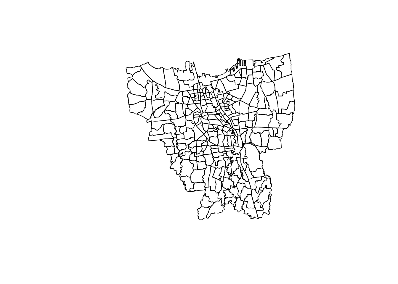
Aspatial Data
Selecting and Renaming the data
Let us first take a look at what the data we are working with looks like.
glimpse(combined_vaccination_data)Rows: 3,216
Columns: 35
$ `KODE KELURAHAN` <chr> NA, "3172051003", "317304…
$ `WILAYAH KOTA` <chr> NA, "JAKARTA UTARA", "JAK…
$ KECAMATAN <chr> NA, "PADEMANGAN", "TAMBOR…
$ KELURAHAN <chr> "TOTAL", "ANCOL", "ANGKE"…
$ SASARAN <dbl> 8941211, 23947, 29381, 29…
$ `BELUM VAKSIN` <dbl> 4441501, 12333, 13875, 18…
$ `JUMLAH\r\nDOSIS 1` <dbl> 4499710, 11614, 15506, 10…
$ `JUMLAH\r\nDOSIS 2` <dbl> 1663218, 4181, 4798, 3658…
$ `TOTAL VAKSIN\r\nDIBERIKAN` <dbl> 6162928, 15795, 20304, 14…
$ `LANSIA\r\nDOSIS 1` <dbl> 502579, 1230, 2012, 865, …
$ `LANSIA\r\nDOSIS 2` <dbl> 440910, 1069, 1729, 701, …
$ `LANSIA TOTAL \r\nVAKSIN DIBERIKAN` <dbl> 943489, 2299, 3741, 1566,…
$ `PELAYAN PUBLIK\r\nDOSIS 1` <dbl> 1052883, 3333, 2586, 2837…
$ `PELAYAN PUBLIK\r\nDOSIS 2` <dbl> 666009, 2158, 1374, 1761,…
$ `PELAYAN PUBLIK TOTAL\r\nVAKSIN DIBERIKAN` <dbl> 1718892, 5491, 3960, 4598…
$ `GOTONG ROYONG\r\nDOSIS 1` <dbl> 56660, 78, 122, 174, 71, …
$ `GOTONG ROYONG\r\nDOSIS 2` <dbl> 38496, 51, 84, 106, 57, 7…
$ `GOTONG ROYONG TOTAL\r\nVAKSIN DIBERIKAN` <dbl> 95156, 129, 206, 280, 128…
$ `TENAGA KESEHATAN\r\nDOSIS 1` <dbl> 76397, 101, 90, 215, 73, …
$ `TENAGA KESEHATAN\r\nDOSIS 2` <dbl> 67484, 91, 82, 192, 67, 3…
$ `TENAGA KESEHATAN TOTAL\r\nVAKSIN DIBERIKAN` <dbl> 143881, 192, 172, 407, 14…
$ `TAHAPAN 3\r\nDOSIS 1` <dbl> 2279398, 5506, 9012, 5408…
$ `TAHAPAN 3\r\nDOSIS 2` <dbl> 446028, 789, 1519, 897, 4…
$ `TAHAPAN 3 TOTAL\r\nVAKSIN DIBERIKAN` <dbl> 2725426, 6295, 10531, 630…
$ `REMAJA\r\nDOSIS 1` <dbl> 531793, 1366, 1684, 1261,…
$ `REMAJA\r\nDOSIS 2` <dbl> 4291, 23, 10, 1, 1, 8, 6,…
$ `REMAJA TOTAL\r\nVAKSIN DIBERIKAN` <dbl> 536084, 1389, 1694, 1262,…
$ Date <chr> "31 Jul 2021", "31 Jul 20…
$ `JUMLAH\r\nDOSIS 3` <dbl> NA, NA, NA, NA, NA, NA, N…
$ `LANSIA\r\nDOSIS 3` <dbl> NA, NA, NA, NA, NA, NA, N…
$ `PELAYAN PUBLIK\r\nDOSIS 3` <dbl> NA, NA, NA, NA, NA, NA, N…
$ `GOTONG ROYONG\r\nDOSIS 3` <dbl> NA, NA, NA, NA, NA, NA, N…
$ `TENAGA KESEHATAN\r\nDOSIS 3` <dbl> NA, NA, NA, NA, NA, NA, N…
$ `TAHAPAN 3\r\nDOSIS 3` <dbl> NA, NA, NA, NA, NA, NA, N…
$ `REMAJA\r\nDOSIS 3` <dbl> NA, NA, NA, NA, NA, NA, N…Of this data, we only need the date, administrative information, and the information pertaining to total vaccinations. As such, we will be selecting the following columns:
[Col 28] Date: The day the data is from
[Col 1] KODE KELURAHAN: Sub-district code
[Col 2] WILAYAH KOTA: City
[Col 3] KECAMATAN: District
[Col 4] KELURAHAN: Sub-District
[Col 5] SASARAN: Target (to be vaccinated)
[Col 6] BELUM VAKSIN: Unvaccinated
[Col 7] JUMLAH DOSIS 1: Number of people with first dose
[Col 8]: JUMLAH DOSIS 2: Number of people with second dose
[Col 29]: JUMLAH DOSIS 3: Number of people with third dose
[Col 9]: TOTAL VAKSIN DIBERIKAN: Total number of vaccine give
vaccination_df_selected <- combined_vaccination_data %>% dplyr::select(c(0:9, 28:29))Now for the ease of reading the data, we will rename the column names accordingly into English.
# Remove newline characters
colnames(vaccination_df_selected) <- colnames(vaccination_df_selected) %>% gsub(pattern="\r\n", replacement=" ")

# Rename columns
vaccination_df <- vaccination_df_selected %>%
  rename(Sub_District_Code = 'KODE KELURAHAN') %>%
  rename(City = 'WILAYAH KOTA') %>%
  rename(District = 'KECAMATAN') %>%
  rename(Sub_District = 'KELURAHAN') %>%
  rename(Target = 'SASARAN') %>%
  rename(Unvaccinated = 'BELUM VAKSIN') %>%
  rename(Dose_1 = 'JUMLAH DOSIS 1') %>%
  rename(Dose_2 = 'JUMLAH DOSIS 2') %>%
  rename(Dose_3 = 'JUMLAH DOSIS 3') %>%
  rename(Tota_Vaccines_Given = 'TOTAL VAKSIN DIBERIKAN')
Select relevant data
As we have done with our geospatial data, we will select only the data from the cities we are studying.
vaccination_df <- vaccination_df %>% filter(City %in% c('JAKARTA BARAT',
                                              'JAKARTA PUSAT',
                                              'JAKARTA SELATAN',
                                              'JAKARTA TIMUR',
                                              'JAKARTA UTARA'))
Joining the data
We can now join all our data into one sf dataframe.
jakarta_vaccination <- left_join(jakarta_boundaries, vaccination_df, by = c("Sub_District" = "Sub_District"))First Look at data
Let us now look at what we have.
tm_shape(jakarta_vaccination) +
  tm_polygons("Dose_1") +
  tm_layout(legend.outside = TRUE,
            legend.outside.position = "left")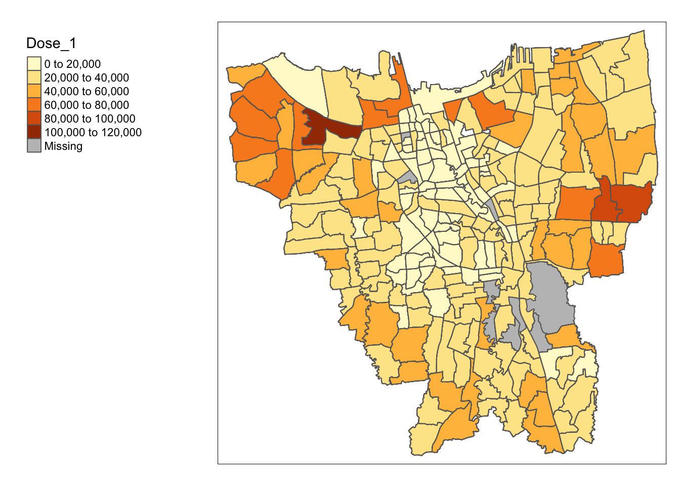
However, we see there are some missing values. This is likely due to mismatched naming of sub-districts, which we will correct in the next section.
Identifying and correcting mismatched sub-district records
vac_subdistrict <- c(vaccination_df$Sub_District)
jkt_subdistrict <- c(jakarta_boundaries$Sub_District)

unique(vac_subdistrict[!(vac_subdistrict %in% jkt_subdistrict)])
[1] "BALE KAMBANG" "HALIM PERDANA KUSUMAH" "JATI PULO"
[4] "KAMPUNG TENGAH" "KERENDANG" "KRAMAT JATI"
[7] "PAL MERIAM" "PINANG RANTI" "RAWA JATI" unique(jkt_subdistrict[!(jkt_subdistrict %in% vac_subdistrict)])[1] "KRENDANG" "RAWAJATI" "TENGAH"
[4] "BALEKAMBANG" "PINANGRANTI" "JATIPULO"
[7] "PALMERIAM" "KRAMATJATI" "HALIM PERDANA KUSUMA"With some inference, we can identify the mismatches and correct them accordingly.
jakarta_boundaries$Sub_District[jakarta_boundaries$Sub_District == 'BALEKAMBANG'] <- 'BALE KAMBANG'
jakarta_boundaries$Sub_District[jakarta_boundaries$Sub_District == 'HALIM PERDANA KUSUMA'] <- 'HALIM PERDANA KUSUMAH'
jakarta_boundaries$Sub_District[jakarta_boundaries$Sub_District == 'JATIPULO'] <- 'JATI PULO'
jakarta_boundaries$Sub_District[jakarta_boundaries$Sub_District == 'TENGAH'] <- 'KAMPUNG TENGAH'
jakarta_boundaries$Sub_District[jakarta_boundaries$Sub_District == 'KRENDANG'] <- 'KERENDANG'
jakarta_boundaries$Sub_District[jakarta_boundaries$Sub_District == 'KRAMATJATI'] <- 'KRAMAT JATI'
jakarta_boundaries$Sub_District[jakarta_boundaries$Sub_District == 'PALMERIAM'] <- 'PAL MERIAM'
jakarta_boundaries$Sub_District[jakarta_boundaries$Sub_District == 'PINANGRANTI'] <- 'PINANG RANTI'
jakarta_boundaries$Sub_District[jakarta_boundaries$Sub_District == 'RAWAJATI'] <- 'RAWA JATI'
Visualising the Data
Now we can do the same again, and we should see no more missing values.
jakarta_vaccination <- left_join(jakarta_boundaries, vaccination_df, by = c("Sub_District" = "Sub_District"))

tm_shape(jakarta_vaccination) +
  tm_polygons("Dose_1") +
  tm_layout(legend.outside = TRUE,
            legend.outside.position = "left")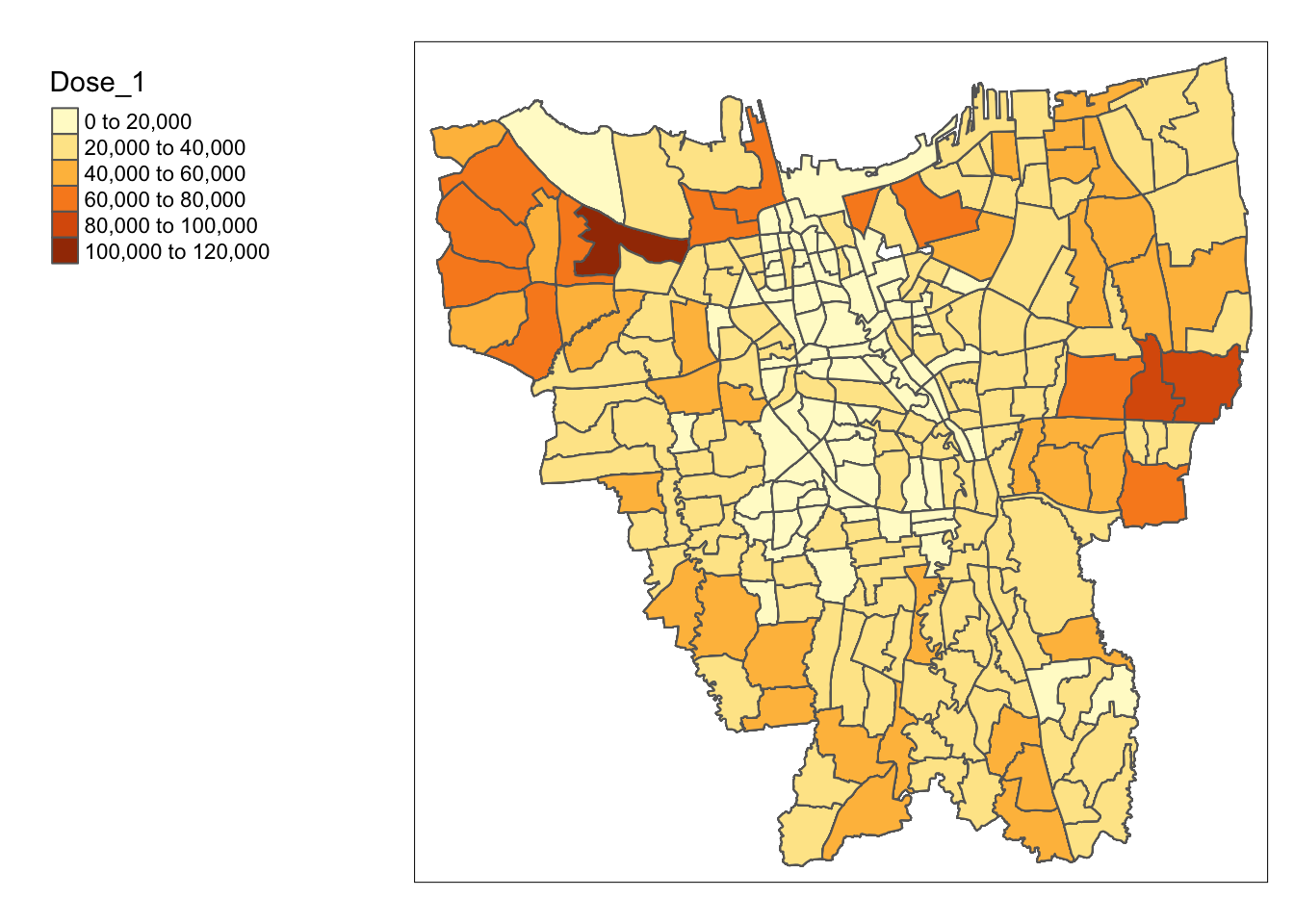
Converting Date to Date object
Lastly, for analysis, we want our data to be in a Date format. So let’s do that conversion.
jakarta_vaccination <- jakarta_vaccination %>%
  mutate(Date = as.Date(Date, format ="%d %b %Y"))
And now, we are ready to start our analysis on our data.
Choropleth Mapping and Analysis
Compute monthly vaccination rate
First, we will replace any NA values with 0 so we do not run into any errors when doing the calculation.
# Remove any NA values
jakarta_vaccination$`Dose_1`[is.na(jakarta_vaccination$`Dose_1`)] = 0
jakarta_vaccination$`Dose_2`[is.na(jakarta_vaccination$`Dose_2`)] = 0
jakarta_vaccination$`Dose_3`[is.na(jakarta_vaccination$`Dose_3`)] = 0
We can then start the computation. Since there are 3 separate Doses of vaccination that we see in our dataset, we will be separating them out into each of their respective rates:
Dose_1_monthly <- jakarta_vaccination %>%
  group_by(Sub_District, Date) %>%
  summarise(Dose_1_Rate = sum(Dose_1) / Target)

Dose_2_monthly <- jakarta_vaccination %>%
  group_by(Sub_District, Date) %>%
  summarise(Dose_2_Rate = sum(Dose_2) / Target)

Dose_3_monthly <- jakarta_vaccination %>% group_by(Sub_District, Date) %>%
  summarise(Dose_3_Rate = sum(Dose_3) / Target)
We can now add these rates as columns in our vaccination_rates sf dataframe.
vaccination_rates <- Dose_1_monthly %>%
  cbind(Dose_2_monthly$Dose_2_Rate, Dose_3_monthly$Dose_3_Rate)

# Rename cols
vaccination_rates <- vaccination_rates %>%
  rename(Dose_2_Rate = Dose_2_monthly.Dose_2_Rate,
         Dose_3_Rate = Dose_3_monthly.Dose_3_Rate)
And now we have our monthly vaccination rates, as previewed below:
glimpse(vaccination_rates)Rows: 3,132
Columns: 6
$ Sub_District <chr> "ANCOL", "ANCOL", "ANCOL", "ANCOL", "ANCOL", "ANCOL", "AN…
$ Date <date> 2021-07-31, 2021-08-31, 2021-09-30, 2021-10-31, 2021-11-…
$ Dose_1_Rate <dbl> 0.4849877, 0.6161941, 0.7207166, 0.7498225, 0.7691986, 0.…
$ Dose_2_Rate <dbl> 0.1745939, 0.3731156, 0.5585668, 0.6056709, 0.6458429, 0.…
$ Dose_3_Rate <dbl> 0.0000000, 0.0000000, 0.0000000, 0.0000000, 0.0000000, 0.…
$ geometry <MULTIPOLYGON [m]> MULTIPOLYGON (((-3621016 69..., MULTIPOLYGON…Since the computation takes very long, let us save the output to an rds format so it does not need to be run again in the future.
saveRDS(vaccination_rates, file="data/rds/vaccination_rates.rds")vaccination_rates <- read_rds("data/rds/vaccination_rates.rds")Choropleth Mapping of Vaccination Rates by Month
We will be using Jenks classification for our choropleth mapping as it is known to be good at finding natural groupings in the data.
jenks_plot <- function(df, var_name) {
  tm_shape(df) +
    tm_fill(var_name,
          n= 6,
          palette = "RdPu",
          style = "jenks") +
    tm_layout(main.title = var_name,
          main.title.position = "center",
          main.title.size = 1.2,
          legend.height = 0.45,
          legend.width = 0.35,
          frame = TRUE) +
    tm_facets(by="Date") +
    tm_borders(alpha = 0.5)
}
And here we have the plotting for each of the respective Doses:
jenks_plot(vaccination_rates, "Dose_1_Rate")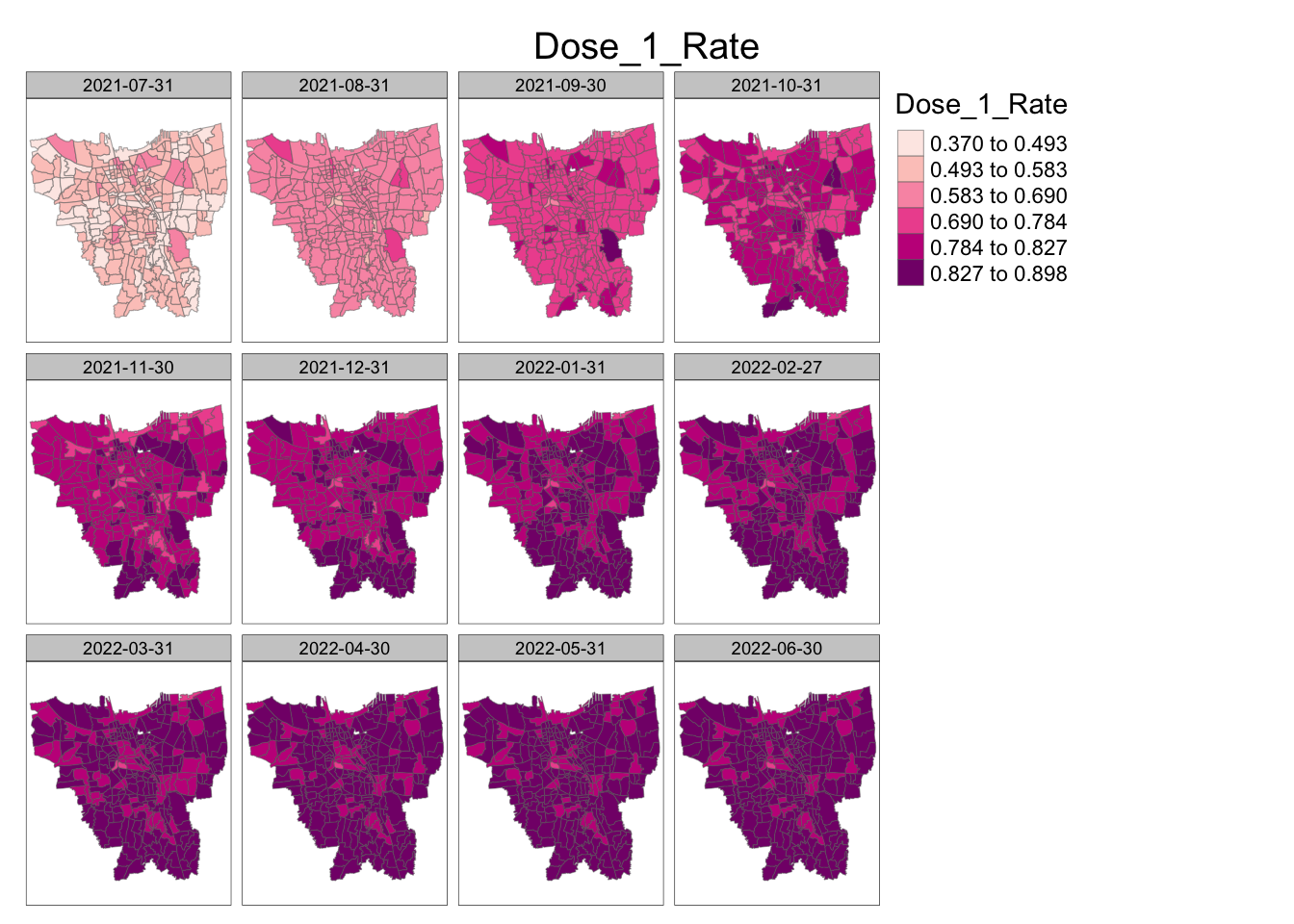
jenks_plot(vaccination_rates, "Dose_2_Rate")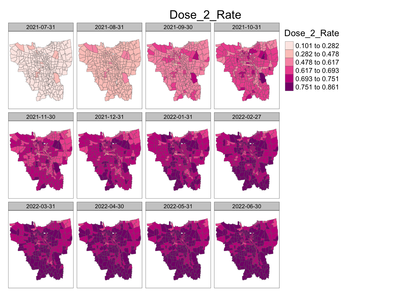
jenks_plot(vaccination_rates, "Dose_3_Rate")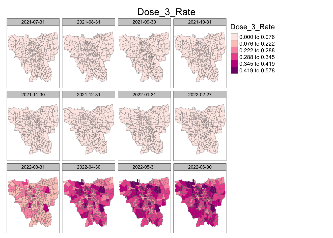
Spatial Pattern Analysis
From these choropleth maps we can see that in general, the rate of vaccination increases as time goes on.
For Dose 1, we can see that over the 12 month period, the rate of vaccination slowly increases throughout the whole country, with the rate increasing a bit faster in the southern and central parts. By the end of the month, the whole of Jakarta has relatively high vaccination rates.
Similar to Dose 1, vaccination rates for Dose 2 steadily increase rather equally throughout Jarkarta during the 12 month period. There is some faster uptake in the southern and central regions.
For Dose 3, for the first 8 months we have a zero vaccination rate throughout Jakarta. This is as the vaccination data was missing initially in these months, most likely because the relatively newer 3rd Dose of the vaccination was likely unavailable until then. However, in March 2022, we see that certain sub-districts near the north border, east border, and come central sub-district have a rather high vaccination rate right from the start. And moving forward, the rate of dose 3 vaccination in these sub-districts and the sub-districts around it are relatively high.
Local Gi* Analysis
We will now use localised spatial statistical analysis in order to further analyse the relationship between vaccination rates and location in Jakarta. For this exercise, we will be using the Local Getis-Ord Gi* Statistic, or Local Gi* for short.]
For this study, we will be using the most recent month of data, June 2022.
vaccination_rates_june22 <- vaccination_rates %>%
  filter(Date == as.Date("2022-06-30"))
Computing Contiguity Weights
wm_idw <- vaccination_rates_june22 %>%
  mutate(nb = st_contiguity(geometry),
         wts = st_inverse_distance(nb, geometry,
                                   scale = 1,
                                   alpha = 1),
         .before = 1)
Compute Local Gi* Statistic
For this statistical test, we will be using a significance level of 0.05. Therefore, we will use nsim=99, and only count results which have a p_sim (p-value) of <0.05.
First, we will set a seed before carrying out simulations so we can always get the same results.
set.seed(415)HCSA_Dose1 <- wm_idw %>%
mutate(local_Gi = local_gstar_perm(
Dose_1_Rate, nb, wt, nsim = 99),
.before = 1) %>%
unnest(local_Gi)
HCSA_Dose2 <- wm_idw %>%
mutate(local_Gi = local_gstar_perm(
Dose_2_Rate, nb, wt, nsim = 99),
.before = 1) %>%
unnest(local_Gi)
HCSA_Dose3 <- wm_idw %>%
mutate(local_Gi = local_gstar_perm(
Dose_3_Rate, nb, wt, nsim = 99),
.before = 1) %>%
unnest(local_Gi)Visualisation
With the calculations done, we can now visualise the Hotspots and Coldspots.
tmap_mode("plot")Visualisation of Hotspots (Gi* > 0) and Coldspots (Gi* < 0)
tm_shape(HCSA_Dose1) +
  tm_fill("gi_star",
          palette = "-RdBu",
          midpoint = 0) +
  tm_borders(alpha = 0.5)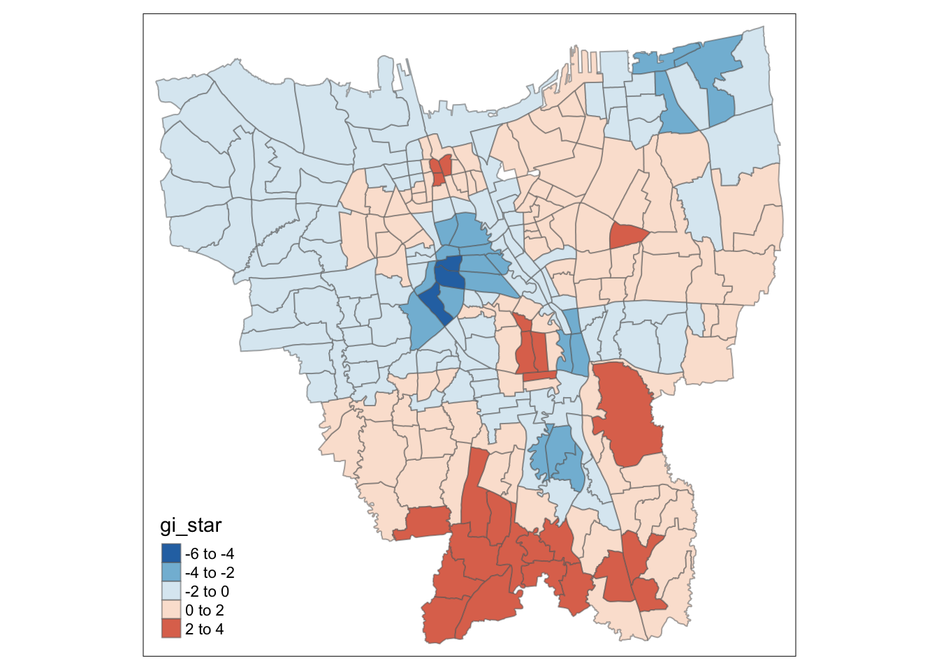
Visualisation of statistically significant values
HCSA_Dose1_sig <- HCSA_Dose1 %>%
  filter(p_sim < 0.05)

tm_shape(HCSA_Dose1) +
  tm_polygons() +
  tm_borders(alpha = 0.5) +
tm_shape(HCSA_Dose1_sig) +
  tm_fill("gi_star",
          palette = "-RdBu",
          midpoint = 0) +
  tm_borders(alpha = 0.5)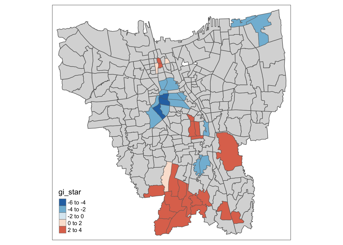
Visualisation of Hotspots (Gi* > 0) and Coldspots (Gi* < 0)
tm_shape(HCSA_Dose2) +
  tm_fill("gi_star",
          palette = "-RdBu",
          midpoint = 0) +
  tm_borders(alpha = 0.5)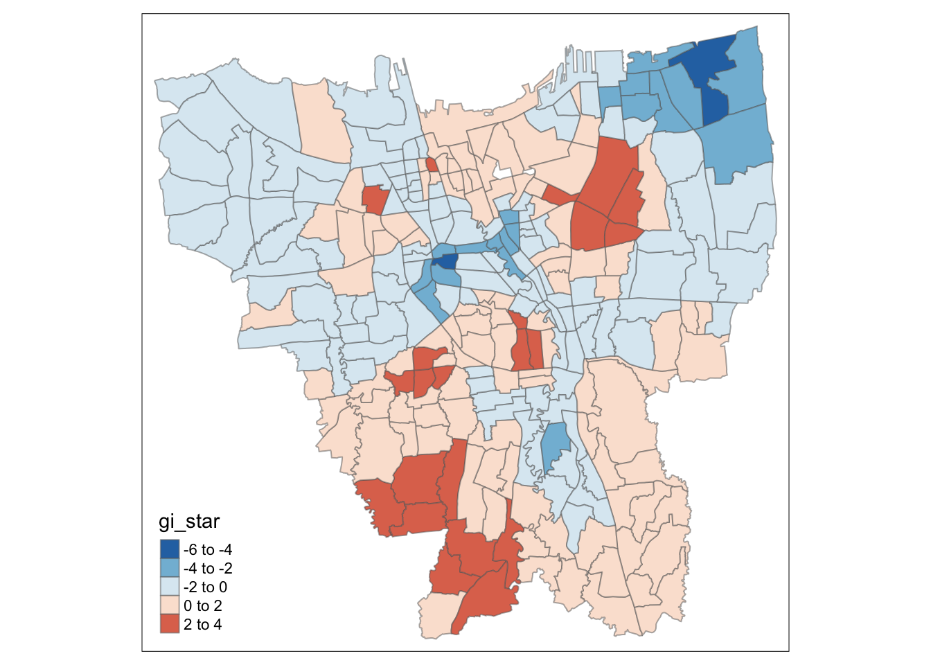
Visualisation of statistically significant values
HCSA_Dose2_sig <- HCSA_Dose2 %>%
  filter(p_sim < 0.05)

tm_shape(HCSA_Dose2) +
  tm_polygons() +
  tm_borders(alpha = 0.5) +
tm_shape(HCSA_Dose2_sig) +
  tm_fill("gi_star",
          palette = "-RdBu",
          midpoint = 0) +
  tm_borders(alpha = 0.5)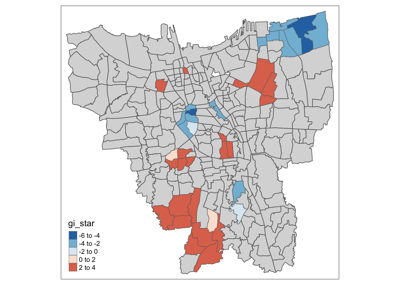
Visualisation of Hotspots (Gi* > 0) and Coldspots (Gi* < 0)
tm_shape(HCSA_Dose3) +
  tm_fill("gi_star",
          palette = "-RdBu",
          midpoint = 0) +
  tm_borders(alpha = 0.5)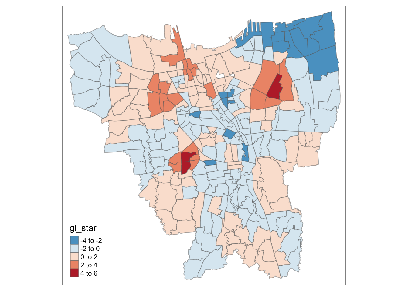
Visualisation of statistically significant values
HCSA_Dose3_sig <- HCSA_Dose3 %>%
  filter(p_sim < 0.05)

tm_shape(HCSA_Dose3) +
  tm_polygons() +
  tm_borders(alpha = 0.5) +
tm_shape(HCSA_Dose3_sig) +
  tm_fill("gi_star",
          palette = "-RdBu",
          midpoint = 0) +
  tm_borders(alpha = 0.5)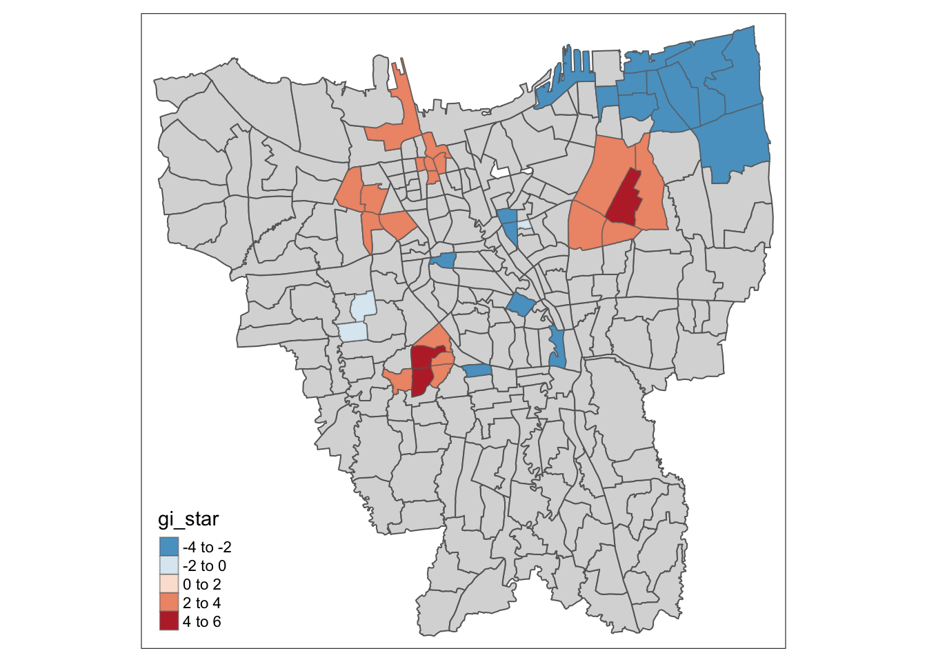
Statistical Analysis
Using these plots, we can now more accurately comment on the statistically significant hot spots and cold spots observed in Jakarta for the respective vaccination dose rates.
For Dose 1 of the vaccine, we see that southern Jakarta is indeed a Hot Spot for Dose 1 vaccines, and experiences a higher than average rate of vaccination. On the other hand, Central Jakarta and some parts of North-Eastern Jakarta appear to be Cold Spots.
Dose 2 has very similar results, with Hot Spots in Southern Jakarta, and Cold Spots in Central and North-Eastern Jakarta. Additionally, there are some other prominent Hot Spots scattered about the center of Jakarta as well.
These scattered Hot Spots about Central Jakarta are present in the Dose 3 analysis as well, but interestingly enough, Southern Jakarta is not a hot spot for Dose 3. If fact, in the visualisation purely Gi* statistic, we can see some parts of Southern Jakarta even have a lower than average rate (but not statistically significant) of vaccination for Dose 3. And once again, North-Eastern Jakarta is also a Cold Spot.
Emerging Hot Spot Analysis (EHSA)
In the previous section, we have done a static analysis on the Hot Spots and Cold Spots in a single month of vaccination data. However, if we want to look at how these patterns emerge and evolve over time, we need to use a spatio-temporal analysis method such as EHSA.
For this analysis, we will be focusing on the vaccination rate of Dose 1, as it has the most vaccinations, and from previous analyses, other Doses 2 and 3 typically follow very similar patterns to Dose 1.
Create Time Series Cube
We first need to convert our data into the suitable data structure for spatio-temporal analysis.
vaccination_rates_st <- vaccination_rates %>%
  as_spacetime(.loc_col="Sub_District", .time_col="Date")
# Verify that it is a space-time cube object
is_spacetime_cube(vaccination_rates_st)[1] TRUECompute Local Gi*
Once again, we will compute the local Gi* statistic. As mentioned above, we will be focusing on the Dose 1 Vaccination Rates. For this test, we will be using a 0.05 significance level (nsim = 99).
# Compute weights
vaccination_rates_nb <- vaccination_rates_st %>%
  activate("geometry") %>%
  mutate(nb = include_self(st_contiguity(geometry)),
         wt = st_inverse_distance(nb, geometry,
                                  scale = 1,
                                  alpha = 1),
         .before = 1) %>%
  set_wts("wt")  %>%
  set_nbs("nb")
# Compute Gi* for Dose 1
gi_stars <- vaccination_rates_nb %>%
group_by(Date) %>%
mutate(gi_star = local_gstar_perm(
Dose_1_Rate, nb, wt, nsim = 99), .before = 1) %>%
tidyr::unnest(gi_star)
gi_stars# A tibble: 3,132 × 15
# Groups: Date [12]
gi_star e_gi var_gi p_value p_sim p_fol…¹ skewn…² kurto…³ Sub_D…⁴
<dbl> <dbl> <dbl> <dbl> <dbl> <dbl> <dbl> <dbl> <chr>
1 1.96 0.00386 0.0000000109 0.0503 0.14 0.07 0.373 -0.183 ANCOL
2 -0.713 0.00381 0.0000000267 0.476 0.42 0.21 0.231 -0.377 ANGKE
3 -4.65 0.00383 0.0000000207 0.00000331 0.02 0.01 0.0745 -0.463 BALE K…
4 -3.46 0.00383 0.0000000154 0.000539 0.04 0.02 -0.336 0.261 BALI M…
5 -1.19 0.00382 0.0000000227 0.236 0.26 0.13 -0.236 -0.424 BAMBU …
6 0.973 0.00382 0.0000000166 0.331 0.36 0.18 0.516 0.531 BANGKA
7 0.990 0.00383 0.0000000196 0.322 0.32 0.16 -0.0215 0.690 BARU
8 -4.88 0.00382 0.0000000177 0.00000104 0.02 0.01 0.242 -0.399 BATU A…
9 -0.970 0.00383 0.0000000165 0.332 0.3 0.15 -0.195 0.0762 BENDUN…
10 -4.12 0.00381 0.0000000118 0.0000372 0.02 0.01 0.351 0.726 BIDARA…
# … with 3,122 more rows, 6 more variables: Date <date>, Dose_1_Rate <dbl>,
# Dose_2_Rate <dbl>, Dose_3_Rate <dbl>, wt <list>, nb <list>, and abbreviated
# variable names ¹p_folded_sim, ²skewness, ³kurtosis, ⁴Sub_DistrictSelect Sub-Districts
For our analysis of emerging hot spots, we will need to select specific Sub Districts to study. As such, let us take a look at some of the data we have.
Let’s first look at the Sub Districts with the highest and lowest vaccination rates at the start of the study period.
# Top 10 highest dose 1 vaccination rates in July 2021
vaccination_rates %>%
  filter(Date == as.Date("2021-07-31")) %>%
  top_n(10, Dose_1_Rate) %>%
  arrange(desc(Dose_1_Rate)) %>%
  dplyr::pull(Sub_District)
[1] "KAMAL MUARA" "HALIM PERDANA KUSUMAH" "KELAPA GADING TIMUR"
[4] "PEGANGSAAN DUA" "KAMPUNG RAWA" "GLODOK"
[7] "ROA MALAKA" "KELAPA GADING BARAT" "MELAWAI"
[10] "MANGGA BESAR" # Top 10 lowest dose 1 vaccination rates in July 2021
vaccination_rates %>%
filter(Date == as.Date("2021-07-31")) %>%
top_n(-10, Dose_1_Rate) %>%
arrange(desc(Dose_1_Rate)) %>%
dplyr::pull(Sub_District) [1] "KLENDER" "CIPINANG BESAR UTARA" "SUKABUMI UTARA"
[4] "BIDARA CINA" "JEMBATAN BESI" "KAMPUNG TENGAH"
[7] "BATU AMPAR" "KEBON MELATI" "PETAMBURAN"
[10] "BALE KAMBANG" And now lets look at the end of the study period.
# Top 10 highest dose 1 vaccination rates in June 2022
vaccination_rates %>%
  filter(Date == as.Date("2022-06-30")) %>%
  top_n(10, Dose_1_Rate) %>%
  arrange(desc(Dose_1_Rate)) %>%
  dplyr::pull(Sub_District)
[1] "HALIM PERDANA KUSUMAH" "SRENGSENG SAWAH" "MANGGARAI SELATAN"
[4] "MALAKA SARI" "GLODOK" "TEBET TIMUR"
[7] "TEBET BARAT" "KELAPA GADING TIMUR" "BARU"
[10] "MALAKA JAYA" # Top 10 lowest dose 1 vaccination rates in June 2022
vaccination_rates %>%
filter(Date == as.Date("2022-06-30")) %>%
top_n(-10, Dose_1_Rate) %>%
arrange(desc(Dose_1_Rate)) %>%
dplyr::pull(Sub_District) [1] "KAMAL" "BIDARA CINA" "KEBON KACANG" "BALE KAMBANG"
[5] "KAMPUNG TENGAH" "GONDANGDIA" "SENAYAN" "KALIBARU"
[9] "PETAMBURAN" "KEBON MELATI" From the top 10 districts with the highest vaccination rate at the begining and end of the vaccination period, we observe the following sub districts in both lists:
HALIM PERDANA KUSUMAH
GLODOK
KELAPA GADING TIMUR
And for the 10 lowest vaccination rates lists, we have these repeated sub districts:
BIDARA CINA
KAMPUNG TENGAH
KEBON MELATI
PETAMBURAN
BALE KAMBANG
For the purpose of our assignment, we must choose 3 Sub Districts to study. As such, let us choose HALIM PERDANA KUSUMAH, GLODOK and BIDARA CINA for our analysis.
Mann-Kendall Test
We can now use the Mann-Kendall Test to observe the temporial patterns in these selected study areas.
hpk <- gi_stars %>%
  ungroup() %>%
  filter(Sub_District == "HALIM PERDANA KUSUMAH") |>
  select(Sub_District, Date, gi_star)
hpk_plot <- ggplot(data = hpk,
aes(x = Date,
y = gi_star)) +
geom_line() +
theme_light()
ggplotly(hpk_plot)hpk %>%
summarise(mk = list(
unclass(
Kendall::MannKendall(gi_star)))) %>%
tidyr::unnest_wider(mk)# A tibble: 1 × 5
tau sl S D varS
<dbl> <dbl> <dbl> <dbl> <dbl>
1 0.758 0.000779 50 66.0 213.glodok <- gi_stars %>%
ungroup() %>%
filter(Sub_District == "GLODOK") |>
select(Sub_District, Date, gi_star)glodok_plot <- ggplot(data = glodok,
aes(x = Date,
y = gi_star)) +
geom_line() +
theme_light()
ggplotly(glodok_plot)glodok %>%
summarise(mk = list(
unclass(
Kendall::MannKendall(gi_star)))) %>%
tidyr::unnest_wider(mk)# A tibble: 1 × 5
tau sl S D varS
<dbl> <dbl> <dbl> <dbl> <dbl>
1 -0.394 0.0865 -26 66.0 213.bc <- gi_stars %>%
ungroup() %>%
filter(Sub_District == "BIDARA CINA") |>
select(Sub_District, Date, gi_star)bc_plot <- ggplot(data = bc,
aes(x = Date,
y = gi_star)) +
geom_line() +
theme_light()
ggplotly(bc_plot)bc %>%
summarise(mk = list(
unclass(
Kendall::MannKendall(gi_star)))) %>%
tidyr::unnest_wider(mk)# A tibble: 1 × 5
tau sl S D varS
<dbl> <dbl> <dbl> <dbl> <dbl>
1 0.545 0.0164 36 66.0 213.Breakdown of Temporal Trends Observed
As expected, our plots support that Halim Perdana Kusumah and Glodok are confirmed to be Hotspots, as they have Gi* Stats > 0 throughout the study period, while Bidara Cina is confirmed to be a Coldspot as it has a negative Gi* Stat throughout the study period.
For Halim Perdana Kusumah, we can observe an upwards trend via the plot. This trend can be counted as statistically significant as the sl (or the p-value) is less than our significance level of 0.05. Hence, we can conclude from the analysis that Halim Perdana Kusumah is an emerging hotspot during this time period.
On the other hand, while Glodok’s Gi* statistic is positive throughout, it does not have a clear upward or downward trend. This is also reflected in its p-value from the Mann-Kendall Test which is greater than our significance level, and hence we are unable to conclude any trend for this Hotspot.
Bidara Cina is another case were we see an upwards trend that is statistically significant (sl value < 0.05). However this is interested, as Bidara Cina is a ColdSpot whose Gi* statistic follows an increasing trend. This suggests that Bidara Cina rate is consistently increasing toward the local average during this time period.
Perform Emerging Hotspot Analysis
Now we will perform EHSA on the whole of Jakarta.
ehsa <- emerging_hotspot_analysis(
  x = vaccination_rates_st,
  .var = "Dose_1_Rate",
  k = 1,
  nsim = 99
)
We can now use ggplot2 to help us look at the distribution of various classes obtained from the analysis.
ggplot(data = ehsa,
       aes(x = classification)) +
  geom_bar(fill="pink")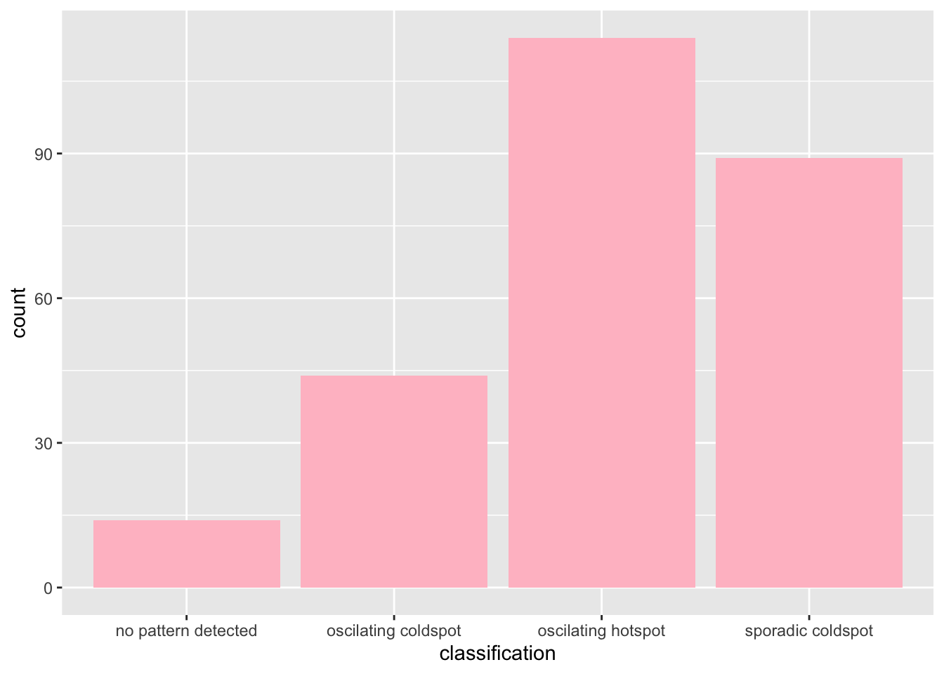
From here, we can see that Oscilating Hotspots are the most common in Jakrata, with Sporadic Coldspots being the second most common.
Visualising EHSA
jakarta_ehsa <- jakarta_boundaries %>%
  left_join(ehsa,
            by = c("Sub_District" = "location"))
ehsa_sig <- jakarta_ehsa %>%
filter(p_value < 0.05)
tm_shape(jakarta_ehsa) +
tm_polygons() +
tm_borders(alpha = 0.5) +
tm_shape(ehsa_sig) +
tm_fill("classification") +
tm_borders(alpha = 0.4)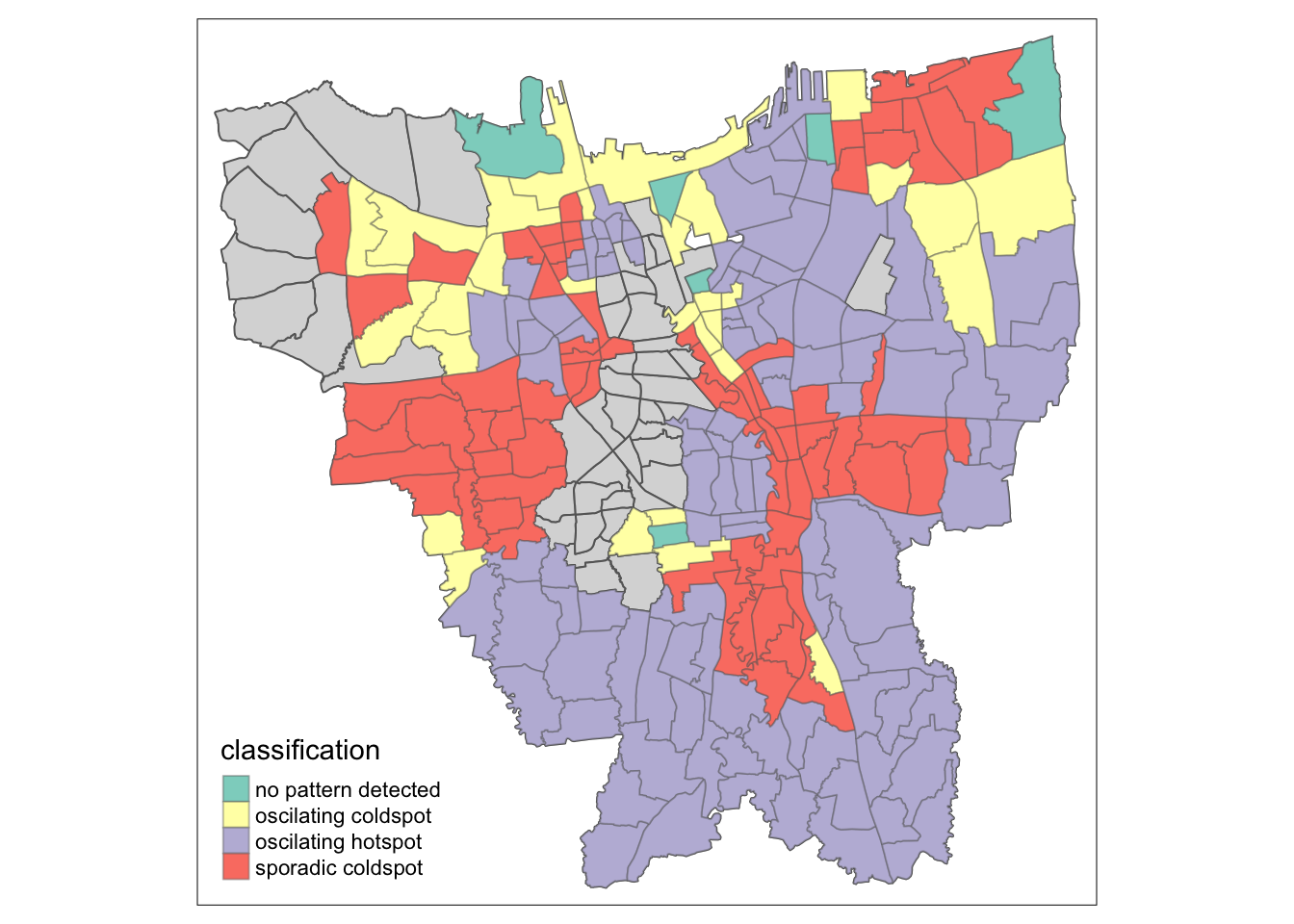
Emerging HotSpot and ColdSpot Analysis
From this simple visualisation, we can now observe at a glance the spatial patterns that emerge over the 12 month time period of this study. Let us break down the area by classification category (with reference to ESRI’s emerging hot spot classification criteria):
Oscillating Hotspots
As seen on the map in purple, Sub districts that are classified in this category are predominantly in the South of Jakarta, as well as in the Central to North-Eastern parts of Jakarta. Such areas, while being predominantly hotspots for most time steps, have also been statistically significant cold spots. Areas classified under this category also spend less than 90% of the time step intervals as statistically significant hot spots.
Sporadic Coldspots
Sub districts falling into this category are marked on the map in red, and predominantly lie in the very North-East of Jakarta, as well as some Central and Western areas of Jakarta. These Sporadic Coldspots are characterised by being a statistically significant Cold spot (for less than 90% of the time step intervals once again) while never being a statistically significant hot spot during the selected study period.
Oscillating Coldspots
Lastly, we have the Oscillating Coldspots, which are shown on the map in yellow. Sub districts under this category lie predominantly in the Northern part of Jakarta. The way these are defined are exactly the same as the aforementioned Oscillating Hotspots, but for cold spots.
Acknowledgements
A big thanks to these senior’s works provided by prof:
Detecting Spatio-Temporal Patterns of COVID-19 in Central Mexico by Xiao Rong Wong.
Take-Home Exercise 1: Analysing and Visualising Spatio-temporal Patterns of COVID-19 in DKI Jakarta, Indonesia by Megan Sim Tze Yen.
As well as Jennifer Poernomo for helping out with the translation for the Vaccination data set <3