pacman::p_load(olsrr, corrplot, ggpubr, sf, spdep, GWmodel, tmap, tidyverse, gtsummary, httr, onemapsgapi, jsonlite, units, matrixStats, rvest, SpatialML, Metrics)Take-Home Exercise 3: Predicting HDB Public Housing Resale Pricies using Geographically Weighted Methods
Introduction
Background and Objective
Housing plays a vital part in our day-to-day lives, and purchasing a home is a significant investment for most people. The cost of housing is influenced by various factors, including global economic conditions and property-specific variables such as its size, fittings, and location.
In this exercise, we will be examining the relationship between HDB Resale Flat Prices and some of these factors, such as the location and age of the resale flat, and proximity to amenities.
Defining the Study Period
For this study, we will be examining a 2-year period of Resale Flat Prices, between Jan 2021 and Dec 2022. We will then conduct geographically weighted regression, and use the months of Jan and Feb of 2023 to test our model.
Data Set Selection
For this exercise, we will be using the below data sets:
Geospatial
- Singapore Master Plan 2019 Subzone Boundary
- Location of Eldercare Centres (from data.gov.sg)
- Location of Hawker Centres (from data.gov.sg)
- Location of MRT Exits (from LTA Data Mall)
- Location of Parks (from data.gov.sg)
- Location of Supermarkets (from data.gov.sg)
- Location of Kindergartens (from data.gov.sg)
- Location of Childcare (from data.gov.sg)
- Location of Bus Stops (from LTA Data Mall)
Aspatial
- HDB Resale Flat Prices (from data.gov.sg)
- Primary Schools as of 2017 (from data.world)
Others
Best Primary Schools 2021 (from salary.sg)
Mall Coordinates WebScraper (from https://github.com/ValaryLim/Mall-Coordinates-Web-Scraper)
Imports
Let us start with importing all the appropriate packages and data sets.
Import Packages
Import Geospatial Data
Singapore Master Plan 2019 Subzone Boundary Dataset
mpsz = st_read(dsn = "data/geospatial/MPSZ-2019", layer = "MPSZ-2019")Reading layer `MPSZ-2019' from data source
`/Users/michelle/Desktop/IS415/shelle-mim/IS415-GAA/Take-home_Exercise/TH3/data/geospatial/MPSZ-2019'
using driver `ESRI Shapefile'
Simple feature collection with 332 features and 6 fields
Geometry type: MULTIPOLYGON
Dimension: XY, XYZ
Bounding box: xmin: 2667.538 ymin: 15748.72 xmax: 56396.44 ymax: 50256.33
z_range: zmin: 0 zmax: 0
Projected CRS: SVY21 / Singapore TMst_crs(mpsz)Coordinate Reference System:
User input: SVY21 / Singapore TM
wkt:
PROJCRS["SVY21 / Singapore TM",
BASEGEOGCRS["SVY21",
DATUM["SVY21",
ELLIPSOID["WGS 84",6378137,298.257223563,
LENGTHUNIT["metre",1]]],
PRIMEM["Greenwich",0,
ANGLEUNIT["degree",0.0174532925199433]],
ID["EPSG",4757]],
CONVERSION["Singapore Transverse Mercator",
METHOD["Transverse Mercator",
ID["EPSG",9807]],
PARAMETER["Latitude of natural origin",1.36666666666667,
ANGLEUNIT["degree",0.0174532925199433],
ID["EPSG",8801]],
PARAMETER["Longitude of natural origin",103.833333333333,
ANGLEUNIT["degree",0.0174532925199433],
ID["EPSG",8802]],
PARAMETER["Scale factor at natural origin",1,
SCALEUNIT["unity",1],
ID["EPSG",8805]],
PARAMETER["False easting",28001.642,
LENGTHUNIT["metre",1],
ID["EPSG",8806]],
PARAMETER["False northing",38744.572,
LENGTHUNIT["metre",1],
ID["EPSG",8807]]],
CS[Cartesian,2],
AXIS["northing (N)",north,
ORDER[1],
LENGTHUNIT["metre",1]],
AXIS["easting (E)",east,
ORDER[2],
LENGTHUNIT["metre",1]],
USAGE[
SCOPE["Cadastre, engineering survey, topographic mapping."],
AREA["Singapore - onshore and offshore."],
BBOX[1.13,103.59,1.47,104.07]],
ID["EPSG",3414]]Elder Care Centers Data Set
eldercare = st_read(dsn = "data/geospatial/Eldercare", layer = "ELDERCARE")Reading layer `ELDERCARE' from data source
`/Users/michelle/Desktop/IS415/shelle-mim/IS415-GAA/Take-home_Exercise/TH3/data/geospatial/Eldercare'
using driver `ESRI Shapefile'
Simple feature collection with 133 features and 18 fields
Geometry type: POINT
Dimension: XY
Bounding box: xmin: 14481.92 ymin: 28218.43 xmax: 41665.14 ymax: 46804.9
Projected CRS: SVY21eldercare <- st_transform(eldercare, 3414)st_crs(eldercare)Coordinate Reference System:
User input: EPSG:3414
wkt:
PROJCRS["SVY21 / Singapore TM",
BASEGEOGCRS["SVY21",
DATUM["SVY21",
ELLIPSOID["WGS 84",6378137,298.257223563,
LENGTHUNIT["metre",1]]],
PRIMEM["Greenwich",0,
ANGLEUNIT["degree",0.0174532925199433]],
ID["EPSG",4757]],
CONVERSION["Singapore Transverse Mercator",
METHOD["Transverse Mercator",
ID["EPSG",9807]],
PARAMETER["Latitude of natural origin",1.36666666666667,
ANGLEUNIT["degree",0.0174532925199433],
ID["EPSG",8801]],
PARAMETER["Longitude of natural origin",103.833333333333,
ANGLEUNIT["degree",0.0174532925199433],
ID["EPSG",8802]],
PARAMETER["Scale factor at natural origin",1,
SCALEUNIT["unity",1],
ID["EPSG",8805]],
PARAMETER["False easting",28001.642,
LENGTHUNIT["metre",1],
ID["EPSG",8806]],
PARAMETER["False northing",38744.572,
LENGTHUNIT["metre",1],
ID["EPSG",8807]]],
CS[Cartesian,2],
AXIS["northing (N)",north,
ORDER[1],
LENGTHUNIT["metre",1]],
AXIS["easting (E)",east,
ORDER[2],
LENGTHUNIT["metre",1]],
USAGE[
SCOPE["Cadastre, engineering survey, topographic mapping."],
AREA["Singapore - onshore and offshore."],
BBOX[1.13,103.59,1.47,104.07]],
ID["EPSG",3414]]Hawker Centers Data Set
hawker_centre = st_read(dsn = "data/geospatial/HawkerCentres/hawker-centres.geojson")Reading layer `hawker-centres' from data source
`/Users/michelle/Desktop/IS415/shelle-mim/IS415-GAA/Take-home_Exercise/TH3/data/geospatial/HawkerCentres/hawker-centres.geojson'
using driver `GeoJSON'
Simple feature collection with 125 features and 2 fields
Geometry type: POINT
Dimension: XYZ
Bounding box: xmin: 103.6974 ymin: 1.272716 xmax: 103.9882 ymax: 1.449217
z_range: zmin: 0 zmax: 0
Geodetic CRS: WGS 84hawker_centre <- st_transform(hawker_centre, 3414)st_crs(hawker_centre)Coordinate Reference System:
User input: EPSG:3414
wkt:
PROJCRS["SVY21 / Singapore TM",
BASEGEOGCRS["SVY21",
DATUM["SVY21",
ELLIPSOID["WGS 84",6378137,298.257223563,
LENGTHUNIT["metre",1]]],
PRIMEM["Greenwich",0,
ANGLEUNIT["degree",0.0174532925199433]],
ID["EPSG",4757]],
CONVERSION["Singapore Transverse Mercator",
METHOD["Transverse Mercator",
ID["EPSG",9807]],
PARAMETER["Latitude of natural origin",1.36666666666667,
ANGLEUNIT["degree",0.0174532925199433],
ID["EPSG",8801]],
PARAMETER["Longitude of natural origin",103.833333333333,
ANGLEUNIT["degree",0.0174532925199433],
ID["EPSG",8802]],
PARAMETER["Scale factor at natural origin",1,
SCALEUNIT["unity",1],
ID["EPSG",8805]],
PARAMETER["False easting",28001.642,
LENGTHUNIT["metre",1],
ID["EPSG",8806]],
PARAMETER["False northing",38744.572,
LENGTHUNIT["metre",1],
ID["EPSG",8807]]],
CS[Cartesian,2],
AXIS["northing (N)",north,
ORDER[1],
LENGTHUNIT["metre",1]],
AXIS["easting (E)",east,
ORDER[2],
LENGTHUNIT["metre",1]],
USAGE[
SCOPE["Cadastre, engineering survey, topographic mapping."],
AREA["Singapore - onshore and offshore."],
BBOX[1.13,103.59,1.47,104.07]],
ID["EPSG",3414]]MRT Data Set
mrt_exit = st_read(dsn = "data/geospatial/TrainStationExit", layer = "Train_Station_Exit_Layer")Reading layer `Train_Station_Exit_Layer' from data source
`/Users/michelle/Desktop/IS415/shelle-mim/IS415-GAA/Take-home_Exercise/TH3/data/geospatial/TrainStationExit'
using driver `ESRI Shapefile'
Simple feature collection with 562 features and 2 fields
Geometry type: POINT
Dimension: XY
Bounding box: xmin: 6134.086 ymin: 27499.7 xmax: 45356.36 ymax: 47865.92
Projected CRS: SVY21mrt_exit <- st_transform(mrt_exit, 3414)st_crs(mrt_exit)Coordinate Reference System:
User input: EPSG:3414
wkt:
PROJCRS["SVY21 / Singapore TM",
BASEGEOGCRS["SVY21",
DATUM["SVY21",
ELLIPSOID["WGS 84",6378137,298.257223563,
LENGTHUNIT["metre",1]]],
PRIMEM["Greenwich",0,
ANGLEUNIT["degree",0.0174532925199433]],
ID["EPSG",4757]],
CONVERSION["Singapore Transverse Mercator",
METHOD["Transverse Mercator",
ID["EPSG",9807]],
PARAMETER["Latitude of natural origin",1.36666666666667,
ANGLEUNIT["degree",0.0174532925199433],
ID["EPSG",8801]],
PARAMETER["Longitude of natural origin",103.833333333333,
ANGLEUNIT["degree",0.0174532925199433],
ID["EPSG",8802]],
PARAMETER["Scale factor at natural origin",1,
SCALEUNIT["unity",1],
ID["EPSG",8805]],
PARAMETER["False easting",28001.642,
LENGTHUNIT["metre",1],
ID["EPSG",8806]],
PARAMETER["False northing",38744.572,
LENGTHUNIT["metre",1],
ID["EPSG",8807]]],
CS[Cartesian,2],
AXIS["northing (N)",north,
ORDER[1],
LENGTHUNIT["metre",1]],
AXIS["easting (E)",east,
ORDER[2],
LENGTHUNIT["metre",1]],
USAGE[
SCOPE["Cadastre, engineering survey, topographic mapping."],
AREA["Singapore - onshore and offshore."],
BBOX[1.13,103.59,1.47,104.07]],
ID["EPSG",3414]]Parks Data Set
parks = st_read(dsn = "data/geospatial/Parks/parks.kml")Reading layer `NATIONALPARKS_New' from data source
`/Users/michelle/Desktop/IS415/shelle-mim/IS415-GAA/Take-home_Exercise/TH3/data/geospatial/Parks/parks.kml'
using driver `KML'
Simple feature collection with 421 features and 2 fields
Geometry type: POINT
Dimension: XYZ
Bounding box: xmin: 103.6929 ymin: 1.214491 xmax: 104.0538 ymax: 1.462094
z_range: zmin: 0 zmax: 0
Geodetic CRS: WGS 84parks <- st_transform(parks, 3414)st_crs(parks)Coordinate Reference System:
User input: EPSG:3414
wkt:
PROJCRS["SVY21 / Singapore TM",
BASEGEOGCRS["SVY21",
DATUM["SVY21",
ELLIPSOID["WGS 84",6378137,298.257223563,
LENGTHUNIT["metre",1]]],
PRIMEM["Greenwich",0,
ANGLEUNIT["degree",0.0174532925199433]],
ID["EPSG",4757]],
CONVERSION["Singapore Transverse Mercator",
METHOD["Transverse Mercator",
ID["EPSG",9807]],
PARAMETER["Latitude of natural origin",1.36666666666667,
ANGLEUNIT["degree",0.0174532925199433],
ID["EPSG",8801]],
PARAMETER["Longitude of natural origin",103.833333333333,
ANGLEUNIT["degree",0.0174532925199433],
ID["EPSG",8802]],
PARAMETER["Scale factor at natural origin",1,
SCALEUNIT["unity",1],
ID["EPSG",8805]],
PARAMETER["False easting",28001.642,
LENGTHUNIT["metre",1],
ID["EPSG",8806]],
PARAMETER["False northing",38744.572,
LENGTHUNIT["metre",1],
ID["EPSG",8807]]],
CS[Cartesian,2],
AXIS["northing (N)",north,
ORDER[1],
LENGTHUNIT["metre",1]],
AXIS["easting (E)",east,
ORDER[2],
LENGTHUNIT["metre",1]],
USAGE[
SCOPE["Cadastre, engineering survey, topographic mapping."],
AREA["Singapore - onshore and offshore."],
BBOX[1.13,103.59,1.47,104.07]],
ID["EPSG",3414]]Supermarkets Data Set
supermarkets = st_read(dsn = "data/geospatial/supermarkets.kml")Reading layer `SUPERMARKETS' from data source
`/Users/michelle/Desktop/IS415/shelle-mim/IS415-GAA/Take-home_Exercise/TH3/data/geospatial/supermarkets.kml'
using driver `KML'
Simple feature collection with 526 features and 2 fields
Geometry type: POINT
Dimension: XYZ
Bounding box: xmin: 103.6258 ymin: 1.24715 xmax: 104.0036 ymax: 1.461526
z_range: zmin: 0 zmax: 0
Geodetic CRS: WGS 84supermarkets <- st_transform(supermarkets, 3414)st_crs(supermarkets)Coordinate Reference System:
User input: EPSG:3414
wkt:
PROJCRS["SVY21 / Singapore TM",
BASEGEOGCRS["SVY21",
DATUM["SVY21",
ELLIPSOID["WGS 84",6378137,298.257223563,
LENGTHUNIT["metre",1]]],
PRIMEM["Greenwich",0,
ANGLEUNIT["degree",0.0174532925199433]],
ID["EPSG",4757]],
CONVERSION["Singapore Transverse Mercator",
METHOD["Transverse Mercator",
ID["EPSG",9807]],
PARAMETER["Latitude of natural origin",1.36666666666667,
ANGLEUNIT["degree",0.0174532925199433],
ID["EPSG",8801]],
PARAMETER["Longitude of natural origin",103.833333333333,
ANGLEUNIT["degree",0.0174532925199433],
ID["EPSG",8802]],
PARAMETER["Scale factor at natural origin",1,
SCALEUNIT["unity",1],
ID["EPSG",8805]],
PARAMETER["False easting",28001.642,
LENGTHUNIT["metre",1],
ID["EPSG",8806]],
PARAMETER["False northing",38744.572,
LENGTHUNIT["metre",1],
ID["EPSG",8807]]],
CS[Cartesian,2],
AXIS["northing (N)",north,
ORDER[1],
LENGTHUNIT["metre",1]],
AXIS["easting (E)",east,
ORDER[2],
LENGTHUNIT["metre",1]],
USAGE[
SCOPE["Cadastre, engineering survey, topographic mapping."],
AREA["Singapore - onshore and offshore."],
BBOX[1.13,103.59,1.47,104.07]],
ID["EPSG",3414]]Kindergartens Data Set
kindergartens = st_read(dsn = "data/geospatial/kindergartens.kml")Reading layer `KINDERGARTENS' from data source
`/Users/michelle/Desktop/IS415/shelle-mim/IS415-GAA/Take-home_Exercise/TH3/data/geospatial/kindergartens.kml'
using driver `KML'
Simple feature collection with 448 features and 2 fields
Geometry type: POINT
Dimension: XYZ
Bounding box: xmin: 103.6887 ymin: 1.247759 xmax: 103.9752 ymax: 1.455452
z_range: zmin: 0 zmax: 0
Geodetic CRS: WGS 84kindergartens <- st_transform(kindergartens, 3414)
st_crs(kindergartens)Coordinate Reference System:
User input: EPSG:3414
wkt:
PROJCRS["SVY21 / Singapore TM",
BASEGEOGCRS["SVY21",
DATUM["SVY21",
ELLIPSOID["WGS 84",6378137,298.257223563,
LENGTHUNIT["metre",1]]],
PRIMEM["Greenwich",0,
ANGLEUNIT["degree",0.0174532925199433]],
ID["EPSG",4757]],
CONVERSION["Singapore Transverse Mercator",
METHOD["Transverse Mercator",
ID["EPSG",9807]],
PARAMETER["Latitude of natural origin",1.36666666666667,
ANGLEUNIT["degree",0.0174532925199433],
ID["EPSG",8801]],
PARAMETER["Longitude of natural origin",103.833333333333,
ANGLEUNIT["degree",0.0174532925199433],
ID["EPSG",8802]],
PARAMETER["Scale factor at natural origin",1,
SCALEUNIT["unity",1],
ID["EPSG",8805]],
PARAMETER["False easting",28001.642,
LENGTHUNIT["metre",1],
ID["EPSG",8806]],
PARAMETER["False northing",38744.572,
LENGTHUNIT["metre",1],
ID["EPSG",8807]]],
CS[Cartesian,2],
AXIS["northing (N)",north,
ORDER[1],
LENGTHUNIT["metre",1]],
AXIS["easting (E)",east,
ORDER[2],
LENGTHUNIT["metre",1]],
USAGE[
SCOPE["Cadastre, engineering survey, topographic mapping."],
AREA["Singapore - onshore and offshore."],
BBOX[1.13,103.59,1.47,104.07]],
ID["EPSG",3414]]Childcare Centers Data Set
childcare = st_read(dsn = "data/geospatial/childcare.geojson")Reading layer `childcare' from data source
`/Users/michelle/Desktop/IS415/shelle-mim/IS415-GAA/Take-home_Exercise/TH3/data/geospatial/childcare.geojson'
using driver `GeoJSON'
Simple feature collection with 1545 features and 2 fields
Geometry type: POINT
Dimension: XYZ
Bounding box: xmin: 103.6824 ymin: 1.248403 xmax: 103.9897 ymax: 1.462134
z_range: zmin: 0 zmax: 0
Geodetic CRS: WGS 84childcare <- st_transform(childcare, 3414)
st_crs(childcare)Coordinate Reference System:
User input: EPSG:3414
wkt:
PROJCRS["SVY21 / Singapore TM",
BASEGEOGCRS["SVY21",
DATUM["SVY21",
ELLIPSOID["WGS 84",6378137,298.257223563,
LENGTHUNIT["metre",1]]],
PRIMEM["Greenwich",0,
ANGLEUNIT["degree",0.0174532925199433]],
ID["EPSG",4757]],
CONVERSION["Singapore Transverse Mercator",
METHOD["Transverse Mercator",
ID["EPSG",9807]],
PARAMETER["Latitude of natural origin",1.36666666666667,
ANGLEUNIT["degree",0.0174532925199433],
ID["EPSG",8801]],
PARAMETER["Longitude of natural origin",103.833333333333,
ANGLEUNIT["degree",0.0174532925199433],
ID["EPSG",8802]],
PARAMETER["Scale factor at natural origin",1,
SCALEUNIT["unity",1],
ID["EPSG",8805]],
PARAMETER["False easting",28001.642,
LENGTHUNIT["metre",1],
ID["EPSG",8806]],
PARAMETER["False northing",38744.572,
LENGTHUNIT["metre",1],
ID["EPSG",8807]]],
CS[Cartesian,2],
AXIS["northing (N)",north,
ORDER[1],
LENGTHUNIT["metre",1]],
AXIS["easting (E)",east,
ORDER[2],
LENGTHUNIT["metre",1]],
USAGE[
SCOPE["Cadastre, engineering survey, topographic mapping."],
AREA["Singapore - onshore and offshore."],
BBOX[1.13,103.59,1.47,104.07]],
ID["EPSG",3414]]Bus Stops Data Set
bus_stops = st_read(dsn = "data/geospatial/BusStop_Feb2023", layer = "BusStop")Reading layer `BusStop' from data source
`/Users/michelle/Desktop/IS415/shelle-mim/IS415-GAA/Take-home_Exercise/TH3/data/geospatial/BusStop_Feb2023'
using driver `ESRI Shapefile'
Simple feature collection with 5159 features and 3 fields
Geometry type: POINT
Dimension: XY
Bounding box: xmin: 3970.122 ymin: 26482.1 xmax: 48284.56 ymax: 52983.82
Projected CRS: SVY21bus_stops <- st_transform(bus_stops, 3414)
st_crs(bus_stops)Coordinate Reference System:
User input: EPSG:3414
wkt:
PROJCRS["SVY21 / Singapore TM",
BASEGEOGCRS["SVY21",
DATUM["SVY21",
ELLIPSOID["WGS 84",6378137,298.257223563,
LENGTHUNIT["metre",1]]],
PRIMEM["Greenwich",0,
ANGLEUNIT["degree",0.0174532925199433]],
ID["EPSG",4757]],
CONVERSION["Singapore Transverse Mercator",
METHOD["Transverse Mercator",
ID["EPSG",9807]],
PARAMETER["Latitude of natural origin",1.36666666666667,
ANGLEUNIT["degree",0.0174532925199433],
ID["EPSG",8801]],
PARAMETER["Longitude of natural origin",103.833333333333,
ANGLEUNIT["degree",0.0174532925199433],
ID["EPSG",8802]],
PARAMETER["Scale factor at natural origin",1,
SCALEUNIT["unity",1],
ID["EPSG",8805]],
PARAMETER["False easting",28001.642,
LENGTHUNIT["metre",1],
ID["EPSG",8806]],
PARAMETER["False northing",38744.572,
LENGTHUNIT["metre",1],
ID["EPSG",8807]]],
CS[Cartesian,2],
AXIS["northing (N)",north,
ORDER[1],
LENGTHUNIT["metre",1]],
AXIS["easting (E)",east,
ORDER[2],
LENGTHUNIT["metre",1]],
USAGE[
SCOPE["Cadastre, engineering survey, topographic mapping."],
AREA["Singapore - onshore and offshore."],
BBOX[1.13,103.59,1.47,104.07]],
ID["EPSG",3414]]Import Aspatial Data
HDB Resale Flat Prices
resale_prices_2017_onwards = read_csv("data/aspatial/resale-flat-prices-based-on-registration-date-from-jan-2017-onwards.csv")Now, we can separate out our data by date into our training and testing data.
resale_prices_2021_22 <- resale_prices_2017_onwards %>%
filter(month < '2023-01') %>%
filter(month > '2020-12')resale_prices_2023 <- resale_prices_2017_onwards %>%
filter(month < '2023-03') %>%
filter(month > '2022-12')Shopping Malls Data Set
malls = read_csv("data/aspatial/mall_coordinates_updated.csv")glimpse(malls)Rows: 184
Columns: 4
$ ...1 <dbl> 0, 1, 2, 3, 4, 5, 6, 7, 8, 9, 10, 11, 12, 13, 14, 15, 16, 17…
$ latitude <dbl> 1.274588, 1.305087, 1.301385, 1.312025, 1.334042, 1.437131, …
$ longitude <dbl> 103.8435, 103.9051, 103.8377, 103.7650, 103.8510, 103.7953, …
$ name <chr> "100 AM", "112 KATONG", "313@SOMERSET", "321 CLEMENTI", "600…malls <- st_as_sf(malls,
coords = c("longitude", "latitude"),
crs=4326) %>%
st_transform(crs = 3414)tmap_mode("plot")
tm_shape(mpsz) +
tm_polygons() +
tm_shape(malls)+
tm_dots()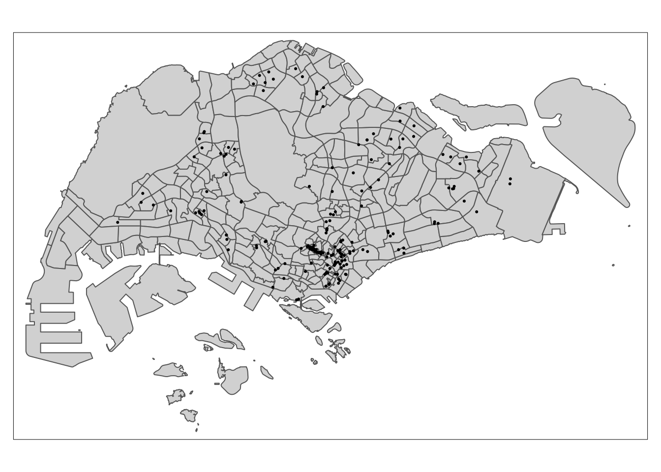
Primary Schools Data Set
pri_schs = read_csv("data/aspatial/primaryschoolsg.csv")glimpse(pri_schs)Rows: 190
Columns: 9
$ Name <chr> "Admiralty Primary School", "Ahmad Ibrahim Pr…
$ Type <chr> "Government", "Government", "Government-aided…
$ GenderMix <chr> "Mixed", "Mixed", "Mixed", "Mixed", "Mixed", …
$ Area <chr> "Woodlands", "Yishun", "Bishan", "Bukit Merah…
$ Zone <chr> "North", "North", "South", "South", "North", …
$ PostalCode <dbl> 738907, 768643, 579646, 159016, 544969, 56978…
$ Latitude <dbl> 1.4427, 1.4333, 1.3603, 1.2913, 1.3913, 1.383…
$ Longitude <dbl> 103.7995, 103.8321, 103.8321, 103.8233, 103.8…
$ PlacestakenuptillPhase2B <dbl> 130, 51, 302, 82, 101, 166, 211, 190, 29, 57,…pri_schs <- pri_schs %>% dplyr::select(c(0:1, 7:8))pri_schs <- st_as_sf(pri_schs,
coords = c("Longitude", "Latitude"),
crs=4326) %>%
st_transform(crs = 3414)tmap_mode("plot")
tm_shape(mpsz) +
tm_polygons() +
tm_shape(pri_schs)+
tm_dots()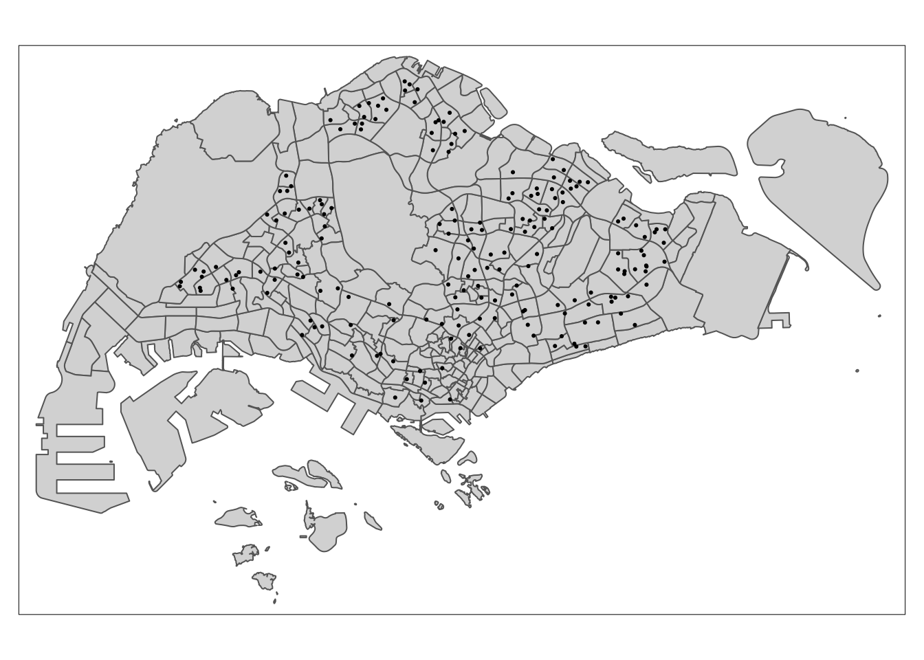
Data Wrangling
Now that we have imported all our data, we can start the data cleaning and transformation process in order to prepare our data for the predictive models we plan to run for it.
Core DataSet: HDB Resale Flat Prices
Firstly, if we look into our darta set, we see that the dataset only provides us the street name and block of the resale flats. In order to turn this into geospatial data, we will need the longitude and latitude of the each flat.
We will be using OneMapSgAPI in order to do this. Let us first write a function that will invoke the API for us and retrieve the longitude and latitude data we need.
geocode <- function(block, streetname) {
base_url <- "https://developers.onemap.sg/commonapi/search"
address <- paste(block, streetname, sep = " ")
query <- list("searchVal" = address,
"returnGeom" = "Y",
"getAddrDetails" = "N",
"pageNum" = "1")
res <- GET(base_url, query = query)
restext<-content(res, as="text")
output <- fromJSON(restext) %>%
as.data.frame %>%
select(results.LATITUDE, results.LONGITUDE)
return(output)
}Now, we can run this function on our datasets in order to populate the dataset. This code takes a long time to load, and as such is saved into and loaded from RDS.
# resale_prices_2021_22$LATITUDE <- 0
# resale_prices_2021_22$LONGITUDE <- 0
#
# for (i in 1:nrow(resale_prices_2021_22)){
# temp_output <- geocode(resale_prices_2021_22[i, 4], resale_prices_2021_22[i, 5])
#
# resale_prices_2021_22$LATITUDE[i] <- temp_output$results.LATITUDE
# resale_prices_2021_22$LONGITUDE[i] <- temp_output$results.LONGITUDE
# }
# resale_prices_2023$LATITUDE <- 0
# resale_prices_2023$LONGITUDE <- 0
#
# for (i in 1:nrow(resale_prices_2023)){
# temp_output <- geocode(resale_prices_2023[i, 4], resale_prices_2023[i, 5])
#
# resale_prices_2023$LATITUDE[i] <- temp_output$results.LATITUDE
# resale_prices_2023$LONGITUDE[i] <- temp_output$results.LONGITUDE
# }We can then do some null checks in order to make sure that our function properly populated our dataframe.
# sum(is.na(resale_prices_2021_22$LATITUDE))
# sum(is.na(resale_prices_2021_22$LONGITUDE))
# sum(resale_prices_2021_22$LATITUDE == 0)
# sum(resale_prices_2021_22$LONGITUDE == 0)# sum(is.na(resale_prices_2023$LATITUDE))
# sum(is.na(resale_prices_2023$LONGITUDE))
# sum(resale_prices_2023$LATITUDE == 0)
# sum(resale_prices_2023$LONGITUDE == 0)# # st_as_sf outputs a simple features data frame
# resale_prices_2021_22_sf <- st_as_sf(resale_prices_2021_22,
# coords = c("LONGITUDE",
# "LATITUDE"),
# # the geographical features are in longitude & latitude, in decimals
# # as such, WGS84 is the most appropriate coordinates system
# crs=4326) %>%
# #afterwards, we transform it to SVY21, our desired CRS
# st_transform(crs = 3414)
# # st_as_sf outputs a simple features data frame
# resale_prices_2023_sf <- st_as_sf(resale_prices_2023,
# coords = c("LONGITUDE",
# "LATITUDE"),
# # the geographical features are in longitude & latitude, in decimals
# # as such, WGS84 is the most appropriate coordinates system
# crs=4326) %>%
# #afterwards, we transform it to SVY21, our desired CRS
# st_transform(crs = 3414)In order to preserve this data, we will now save it to rds.
# saveRDS(resale_prices_2021_22_sf, file="data/rds/resale_prices_2021_22_sf.rds")
# saveRDS(resale_prices_2023_sf, file="data/rds/resale_prices_2023_sf.rds")And now we can load it.
resale_prices_2021_22_sf <- read_rds("data/rds/resale_prices_2021_22_sf.rds")
resale_prices_2023_sf <- read_rds("data/rds/resale_prices_2023_sf.rds")We can now display our data on the map.
tmap_mode("plot")
tm_shape(mpsz) +
tm_polygons() +
tm_shape(resale_prices_2021_22_sf)+
tm_dots(col = "resale_price",
size = 0.01,
border.col = "black",
border.lwd = 0.5) +
tmap_options(check.and.fix = TRUE) +
tm_view(set.zoom.limits = c(11, 16)) +
tm_layout(legend.outside = TRUE)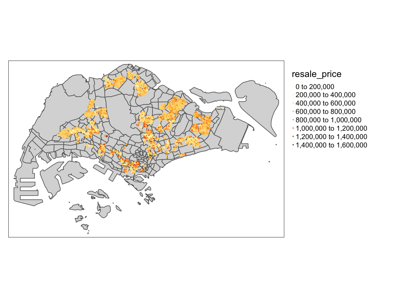
tmap_mode("plot")
tm_shape(mpsz) +
tm_polygons() +
tm_shape(resale_prices_2023_sf)+
tm_dots(col = "resale_price",
size = 0.01,
border.col = "black",
border.lwd = 0.5) +
tmap_options(check.and.fix = TRUE) +
tm_view(set.zoom.limits = c(11, 16)) +
tm_layout(legend.outside = TRUE)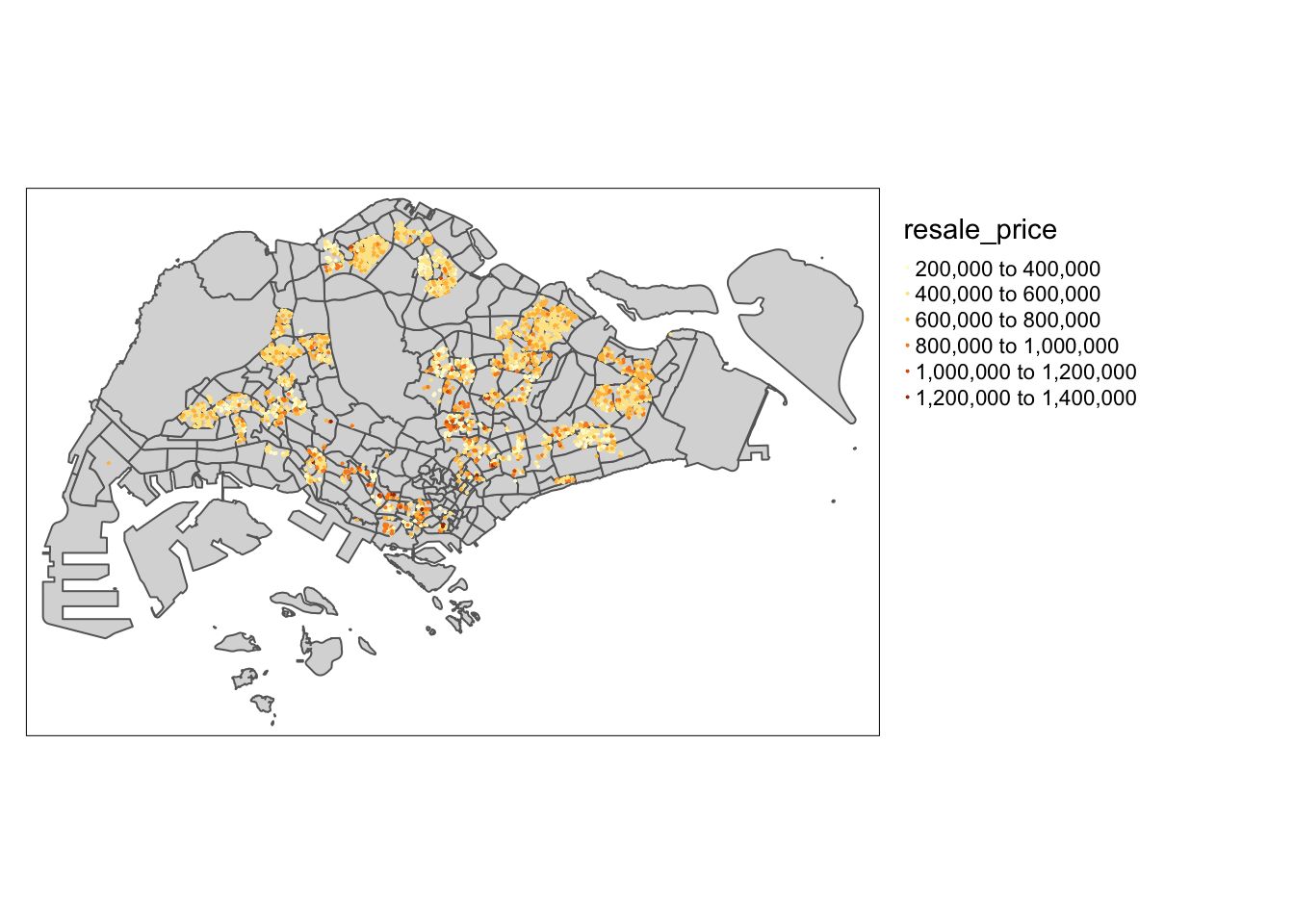
Geospatial Data
Now that we have transformed our HDB Resale Price data, we can move on to creating some of the other metrics we want to look at in our analysis.
Proximity to CBD
In order to get the distance to the CBD, we must first identify where the CBD is, then find its centre. We can then calculate the distance. Let us start by looking at the Planning Areas in our dataset.
unique(mpsz$PLN_AREA_N) [1] "MARINA EAST" "RIVER VALLEY"
[3] "SINGAPORE RIVER" "WESTERN ISLANDS"
[5] "MUSEUM" "MARINE PARADE"
[7] "SOUTHERN ISLANDS" "BUKIT MERAH"
[9] "DOWNTOWN CORE" "STRAITS VIEW"
[11] "QUEENSTOWN" "OUTRAM"
[13] "MARINA SOUTH" "ROCHOR"
[15] "KALLANG" "TANGLIN"
[17] "NEWTON" "CLEMENTI"
[19] "BEDOK" "PIONEER"
[21] "JURONG EAST" "ORCHARD"
[23] "GEYLANG" "BOON LAY"
[25] "BUKIT TIMAH" "NOVENA"
[27] "TOA PAYOH" "TUAS"
[29] "JURONG WEST" "SERANGOON"
[31] "BISHAN" "TAMPINES"
[33] "BUKIT BATOK" "HOUGANG"
[35] "CHANGI BAY" "PAYA LEBAR"
[37] "ANG MO KIO" "PASIR RIS"
[39] "BUKIT PANJANG" "TENGAH"
[41] "SELETAR" "SUNGEI KADUT"
[43] "YISHUN" "MANDAI"
[45] "PUNGGOL" "CHOA CHU KANG"
[47] "SENGKANG" "CHANGI"
[49] "CENTRAL WATER CATCHMENT" "SEMBAWANG"
[51] "WESTERN WATER CATCHMENT" "WOODLANDS"
[53] "NORTH-EASTERN ISLANDS" "SIMPANG"
[55] "LIM CHU KANG" As we can see, we already have the Downtown Core as a Planning Area. And as said by the Urban Redevelopment Authority, “The Downtown Core Planning Area is the economic and cultural heart of Singapore”, and encompasses the Central Business District. As such, we will be using the centroid of the
# Extract Downtown core
downtown_core <- mpsz %>%
filter(PLN_AREA_N == "DOWNTOWN CORE") %>%
st_combine()# Get Centroid
downtown_core_centroid <- downtown_core %>%
st_centroid()
downtown_core_centroidGeometry set for 1 feature
Geometry type: POINT
Dimension: XY
Bounding box: xmin: 30468.27 ymin: 29912.14 xmax: 30468.27 ymax: 29912.14
Projected CRS: SVY21 / Singapore TM# Plot
tmap_mode("plot")
tm_shape(mpsz) +
tm_polygons() +
tmap_options(check.and.fix = TRUE) +
tm_shape(downtown_core) +
tm_fill(col = "pink") +
tm_shape(downtown_core_centroid) +
tm_dots() +
tm_view(set.zoom.limits = c(11, 16))
Great! We now have our centroid that we can use to calculate the distance to. We can now use the coordinates of our centroid and makew an sf dataframe for later use.
st_coordinates(downtown_core_centroid) X Y
[1,] 30468.27 29912.14lat <- 30335.19
lng <- 129721.45
downtown_core_centroid_sf <- data.frame(lat, lng) %>%
st_as_sf(coords = c("lng", "lat"), crs=3414)With that done, we can now calculate the Proximity to CBD. But before we do that, we need to change our centroid into an sf dataframe for comparison. We will do this altogether for all the seperate data sets in a later section for simplicity and data consistency.
Proximity to Good Primary School
For this metric, there were no readily available data sets. As such, we will attain this information via webscraping. We will be scraping https://www.salary.sg/2021/best-primary-schools-2021-by-popularity/, which provides a ranking of the Best Primary Schools by popularity.
url <- "https://www.salary.sg/2021/best-primary-schools-2021-by-popularity/"
good_pri <- data.frame()
schools <- read_html(url) %>%
html_nodes(xpath = paste('//*[@id="post-3068"]/div[3]/div/div/ol/li') ) %>%
html_text()
for (i in (schools)){
sch_name <- toupper(gsub(" – .*","",i))
sch_name <- gsub("\\(PRIMARY SECTION)","",sch_name)
sch_name <- trimws(sch_name)
new_row <- data.frame(pri_sch_name=sch_name)
# Add the row
good_pri <- rbind(good_pri, new_row)
}Since we are looking out for good primary schools, let us select the first 20 results that we will find the proximity to for our analysis.
top_pri_sch <- head(good_pri, 20)Since we already have the coordinates from our primary school data, we can left_join in order to add the coordinates to our list of top primary schools. But first, we need to do a little data preparation to make sure the columns match.
top_pri_sch$pri_sch_name[!tolower(top_pri_sch$pri_sch_name) %in% tolower(pri_schs$Name)][1] "CHIJ ST. NICHOLAS GIRLS’ SCHOOL" "CATHOLIC HIGH SCHOOL"
[3] "ST. HILDA’S PRIMARY SCHOOL" "HOLY INNOCENTS’ PRIMARY SCHOOL"
[5] "METHODIST GIRLS’ SCHOOL (PRIMARY)"It seems the issue lies with different apostrophes being used, as well as Catholic High School. We can easily change those to match our primary school dataset.
top_pri_sch$pri_sch_name <- gsub('’', "'", top_pri_sch$pri_sch_name)
top_pri_sch$pri_sch_name[top_pri_sch$pri_sch_name == 'CATHOLIC HIGH SCHOOL'] <- 'CATHOLIC HIGH SCHOOL (PRIMARY)'Now that that is settled, we can join the data to get out coordinates.
# Convert to lowercase for easy comparison
top_pri_sch$pri_sch_name <- tolower(top_pri_sch$pri_sch_name)
# Function to do our join for us
join_lowercase_name <- function(left,right){
right$Name <- tolower(right$Name)
inner_join(left,right,by=c("pri_sch_name" = "Name"))
}
top_pri_sch <- join_lowercase_name(top_pri_sch, pri_schs) top_pri_sch <- st_as_sf(top_pri_sch, crs=3414)
st_crs(top_pri_sch)Coordinate Reference System:
User input: EPSG:3414
wkt:
PROJCRS["SVY21 / Singapore TM",
BASEGEOGCRS["SVY21",
DATUM["SVY21",
ELLIPSOID["WGS 84",6378137,298.257223563,
LENGTHUNIT["metre",1]]],
PRIMEM["Greenwich",0,
ANGLEUNIT["degree",0.0174532925199433]],
ID["EPSG",4757]],
CONVERSION["Singapore Transverse Mercator",
METHOD["Transverse Mercator",
ID["EPSG",9807]],
PARAMETER["Latitude of natural origin",1.36666666666667,
ANGLEUNIT["degree",0.0174532925199433],
ID["EPSG",8801]],
PARAMETER["Longitude of natural origin",103.833333333333,
ANGLEUNIT["degree",0.0174532925199433],
ID["EPSG",8802]],
PARAMETER["Scale factor at natural origin",1,
SCALEUNIT["unity",1],
ID["EPSG",8805]],
PARAMETER["False easting",28001.642,
LENGTHUNIT["metre",1],
ID["EPSG",8806]],
PARAMETER["False northing",38744.572,
LENGTHUNIT["metre",1],
ID["EPSG",8807]]],
CS[Cartesian,2],
AXIS["northing (N)",north,
ORDER[1],
LENGTHUNIT["metre",1]],
AXIS["easting (E)",east,
ORDER[2],
LENGTHUNIT["metre",1]],
USAGE[
SCOPE["Cadastre, engineering survey, topographic mapping."],
AREA["Singapore - onshore and offshore."],
BBOX[1.13,103.59,1.47,104.07]],
ID["EPSG",3414]]Proximity and Frequency Calculations
With all our data prepared and ready for use, we can now move on to calculations.
Let us now write functions to calculate the proximity and frequency of the relevant features to our resale price data:
proximity <- function(df1, df2, varname) {
dist_matrix <- st_distance(df1, df2) %>%
drop_units()
df1[,varname] <- rowMins(dist_matrix)
return(df1)
}
num_radius <- function(df1, df2, varname, radius) {
dist_matrix <- st_distance(df1, df2) %>%
drop_units() %>%
as.data.frame()
df1[,varname] <- rowSums(dist_matrix <= radius)
return(df1)
}With these, we can do our calculations all at once.
# resale_full_details_2021_22_sf <-
# proximity(resale_prices_2021_22_sf, downtown_core_centroid_sf, "PROX_CBD") %>%
# proximity(., eldercare, "PROX_ELDERCARE") %>%
# proximity(., hawker_centre, "PROX_HAWKER_CENTRE") %>%
# proximity(., mrt_exit, "PROX_MRT") %>%
# proximity(., parks, "PROX_PARK") %>%
# proximity(., top_pri_sch, "PROX_GOOD_PRI_SCH") %>%
# proximity(., malls, "PROX_MALL") %>%
# proximity(., supermarkets, "PROX_SUPERMARKET")
#
# resale_full_details_2023_sf <-
# proximity(resale_prices_2023_sf, downtown_core_centroid_sf, "PROX_CBD") %>%
# proximity(., eldercare, "PROX_ELDERCARE") %>%
# proximity(., hawker_centre, "PROX_HAWKER_CENTRE") %>%
# proximity(., mrt_exit, "PROX_MRT") %>%
# proximity(., parks, "PROX_PARK") %>%
# proximity(., top_pri_sch, "PROX_GOOD_PRI_SCH") %>%
# proximity(., malls, "PROX_MALL") %>%
# proximity(., supermarkets, "PROX_SUPERMARKET")# resale_full_details_2021_22_sf <-
# num_radius(resale_prices_2021_22_sf, kindergartens, "NUM_KINDERGARTEN", 350) %>%
# num_radius(., childcare, "NUM_CHILDCARE", 350) %>%
# num_radius(., bus_stops, "NUM_BUS_STOP", 350) %>%
# num_radius(., pri_schs, "NUM_PRI_SCH", 1000)
#
# resale_full_details_2023_sf <-
# num_radius(resale_prices_2023_sf, kindergartens, "NUM_KINDERGARTEN", 350) %>%
# num_radius(., childcare, "NUM_CHILDCARE", 350) %>%
# num_radius(., bus_stops, "NUM_BUS_STOP", 350) %>%
# num_radius(., pri_schs, "NUM_PRI_SCH", 1000)Since these calculations take a while to load, lets save and load everything from RDS.
# saveRDS(resale_full_details_2021_22_sf, file="data/rds/resale_full_details_2021_22_sf.rds")
# saveRDS(resale_full_details_2023_sf, file="data/rds/resale_full_details_2023_sf.rds")
resale_full_details_2021_22_sf <- read_rds("data/rds/resale_full_details_2021_22_sf.rds")
resale_full_details_2023_sf <- read_rds("data/rds/resale_full_details_2023_sf.rds")Data Preparation
Before we start on our linear regression, we first need to transform our data into an appropriate format that the model for the regression model to interpret. As such, we will be changing all our categorical variables into numerical variables via encoding.
Encoding Variables
Let us first look at what we are working with.
glimpse(resale_full_details_2021_22_sf)Rows: 55,817
Columns: 24
$ month <chr> "2021-01", "2021-01", "2021-01", "2021-01", "2021-…
$ town <chr> "ANG MO KIO", "ANG MO KIO", "ANG MO KIO", "ANG MO …
$ flat_type <chr> "2 ROOM", "2 ROOM", "3 ROOM", "3 ROOM", "3 ROOM", …
$ block <chr> "170", "170", "331", "534", "561", "170", "463", "…
$ street_name <chr> "ANG MO KIO AVE 4", "ANG MO KIO AVE 4", "ANG MO KI…
$ storey_range <chr> "01 TO 03", "07 TO 09", "04 TO 06", "04 TO 06", "0…
$ floor_area_sqm <dbl> 45, 45, 68, 68, 68, 60, 68, 68, 60, 73, 67, 67, 68…
$ flat_model <chr> "Improved", "Improved", "New Generation", "New Gen…
$ lease_commence_date <dbl> 1986, 1986, 1981, 1980, 1980, 1986, 1980, 1981, 19…
$ remaining_lease <chr> "64 years 01 month", "64 years 01 month", "59 year…
$ resale_price <dbl> 211000, 225000, 260000, 265000, 265000, 268000, 26…
$ geometry <POINT [m]> POINT (28346.43 39555.53), POINT (28346.43 3…
$ PROX_CBD <dbl> 101793.46, 101793.46, 100092.40, 99828.46, 99384.9…
$ PROX_ELDERCARE <dbl> 429.68375, 429.68375, 412.40581, 1008.60569, 683.4…
$ PROX_HAWKER_CENTRE <dbl> 314.3604, 314.3604, 356.0478, 146.7193, 307.8475, …
$ PROX_MRT <dbl> 73.66065, 73.66065, 818.28864, 668.50386, 889.4625…
$ PROX_PARK <dbl> 303.1924, 303.1924, 358.0379, 554.3379, 817.5539, …
$ PROX_GOOD_PRI_SCH <dbl> 262.1063, 262.1063, 957.1154, 409.3479, 602.7432, …
$ PROX_MALL <dbl> 1439.9090, 1439.9090, 826.9463, 829.6281, 1012.796…
$ PROX_SUPERMARKET <dbl> 3.413032e+02, 3.413032e+02, 4.369613e+02, 1.592391…
$ NUM_KINDERGARTEN <dbl> 1, 1, 1, 1, 1, 1, 2, 1, 1, 0, 2, 1, 0, 1, 0, 2, 1,…
$ NUM_CHILDCARE <dbl> 4, 4, 2, 2, 4, 4, 5, 2, 4, 2, 3, 2, 2, 2, 3, 4, 2,…
$ NUM_BUS_STOP <dbl> 3, 3, 7, 11, 8, 3, 6, 9, 3, 4, 5, 4, 6, 9, 9, 5, 4…
$ NUM_PRI_SCH <dbl> 3, 3, 3, 4, 4, 3, 5, 3, 3, 1, 3, 2, 3, 5, 2, 3, 2,…While all our freshly calculated data looks good, we can see some of the variables from our resale dataset still need to further processed, namely storey_range and remaining_lease. We also have to use lease_commence_date and month in order to determine the age of the unit.
Remaining lease is the easiest to fix, we can simplify it to just the number of years left, and cast it to a number.
resale_full_details_2021_22_sf$remaining_lease <- as.numeric(
word(resale_full_details_2021_22_sf$remaining_lease, 1))
resale_full_details_2023_sf$remaining_lease <- as.numeric(
word(resale_full_details_2023_sf$remaining_lease, 1))Storey Range is slightly more difficult, as we will have to transform the range into an ordinal variable.
unique(resale_full_details_2021_22_sf$storey_range) [1] "01 TO 03" "07 TO 09" "04 TO 06" "10 TO 12" "13 TO 15" "16 TO 18"
[7] "19 TO 21" "22 TO 24" "28 TO 30" "25 TO 27" "34 TO 36" "31 TO 33"
[13] "37 TO 39" "43 TO 45" "40 TO 42" "46 TO 48" "49 TO 51"However, we can see that the storey ranges fall very nicely into ranges of 3. As such, we can transform them into ordinal values by taking the last word in the string, converting it into a number, then dividing by 3.
resale_full_details_2021_22_sf$storey_range <- (as.numeric(
word(resale_full_details_2021_22_sf$storey_range, -1)) / 3)
resale_full_details_2023_sf$storey_range <- (as.numeric(
word(resale_full_details_2023_sf$storey_range, -1)) / 3)Lastly, we have the Age of Unit to calculate. We can get this value in years by taking the month minus the lease_commence_date.
resale_full_details_2021_22_sf <- resale_full_details_2021_22_sf %>%
add_column(age_of_unit = NA) %>%
mutate(age_of_unit = (
as.numeric(substr(resale_full_details_2021_22_sf$month, 1, 4)) -
as.numeric(resale_full_details_2021_22_sf$lease_commence_date)))
resale_full_details_2023_sf <- resale_full_details_2023_sf %>%
add_column(age_of_unit = NA) %>%
mutate(age_of_unit = (
as.numeric(substr(resale_full_details_2023_sf$month, 1, 4)) -
as.numeric(resale_full_details_2023_sf$lease_commence_date)))Let’s just double check that all our calculations went well:
sum(is.na(resale_full_details_2021_22_sf$age_of_unit))[1] 0sum(is.na(resale_full_details_2023_sf$age_of_unit))[1] 0Separate into Sub-Markets
Now that we have encoded all the necessary values, we can drop all other columns. However, before we do this, we need to separate our data into our 3 sub-markets of interest: 3-room, 4-room and 5-room flats.
three_room_2021_22_sf <- resale_full_details_2021_22_sf %>%
filter(flat_type == '3 ROOM')
four_room_2021_22_sf <- resale_full_details_2021_22_sf %>%
filter(flat_type == '4 ROOM')
five_room_2021_22_sf <- resale_full_details_2021_22_sf %>%
filter(flat_type == '5 ROOM')
three_room_2023_sf <- resale_full_details_2023_sf %>%
filter(flat_type == '3 ROOM')
four_room_2023_sf <- resale_full_details_2023_sf %>%
filter(flat_type == '4 ROOM')
five_room_2023_sf <- resale_full_details_2023_sf %>%
filter(flat_type == '5 ROOM')Remove Unnecessary Columns
Now that we have encoded all the necessary values, we can drop all other columns before saving this to rds for us to work on in our regression section later.
three_room_2021_22_sf <- three_room_2021_22_sf %>%
dplyr::select(c(6:7, 10:25))
four_room_2021_22_sf <- four_room_2021_22_sf %>%
dplyr::select(c(6:7, 10:25))
five_room_2021_22_sf <- five_room_2021_22_sf %>%
dplyr::select(c(6:7, 10:25))
three_room_2023_sf <- three_room_2023_sf %>%
dplyr::select(c(6:7, 10:25))
four_room_2023_sf <- four_room_2023_sf %>%
dplyr::select(c(6:7, 10:25))
five_room_2023_sf <- five_room_2023_sf %>%
dplyr::select(c(6:7, 10:25))# saveRDS(three_room_2021_22_sf, file="data/rds/three_room_2021_22_sf.rds")
# saveRDS(four_room_2021_22_sf, file="data/rds/four_room_2021_22_sf.rds")
# saveRDS(five_room_2021_22_sf, file="data/rds/five_room_2021_22_sf.rds")
#
# saveRDS(three_room_2023_sf, file="data/rds/three_room_2023_sf.rds")
# saveRDS(four_room_2023_sf, file="data/rds/four_room_2023_sf.rds")
# saveRDS(five_room_2023_sf, file="data/rds/five_room_2023_sf.rds")
three_room_2021_22_sf <- read_rds("data/rds/three_room_2021_22_sf.rds")
four_room_2021_22_sf <- read_rds("data/rds/four_room_2021_22_sf.rds")
five_room_2021_22_sf <- read_rds("data/rds/five_room_2021_22_sf.rds")
three_room_2023_sf <- read_rds("data/rds/three_room_2023_sf.rds")
four_room_2023_sf <- read_rds("data/rds/four_room_2023_sf.rds")
five_room_2023_sf <- read_rds("data/rds/five_room_2023_sf.rds")Exploratory Data Analysis
Statistical Visualisation
Resale Price
Before we jump into our analysis, let us first do some visualization on our test data, starting with our resale prices.
# Remove scientific notation from our graphs
options(scipen = 999)ggplot(data=three_room_2021_22_sf, aes(x=`resale_price`)) +
geom_histogram(bins=20, color="black", fill="pink") +
labs(title = "Distribution of Resale Prices for 3 Room Flats (2021 - 2022)",
x = "Resale Prices",
y = 'Frequency') +
scale_x_continuous(labels = scales::comma) +
scale_y_continuous(labels = scales::comma)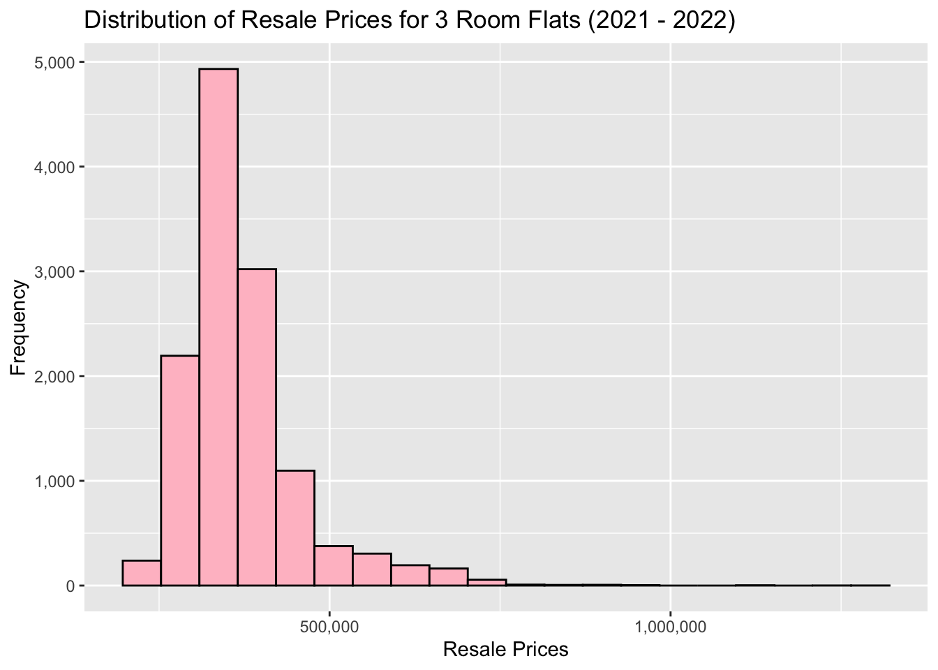
ggplot(data = three_room_2021_22_sf, aes(x = '', y = resale_price)) +
geom_boxplot() +
labs(x='', y='3 Room Resale Flat Prices')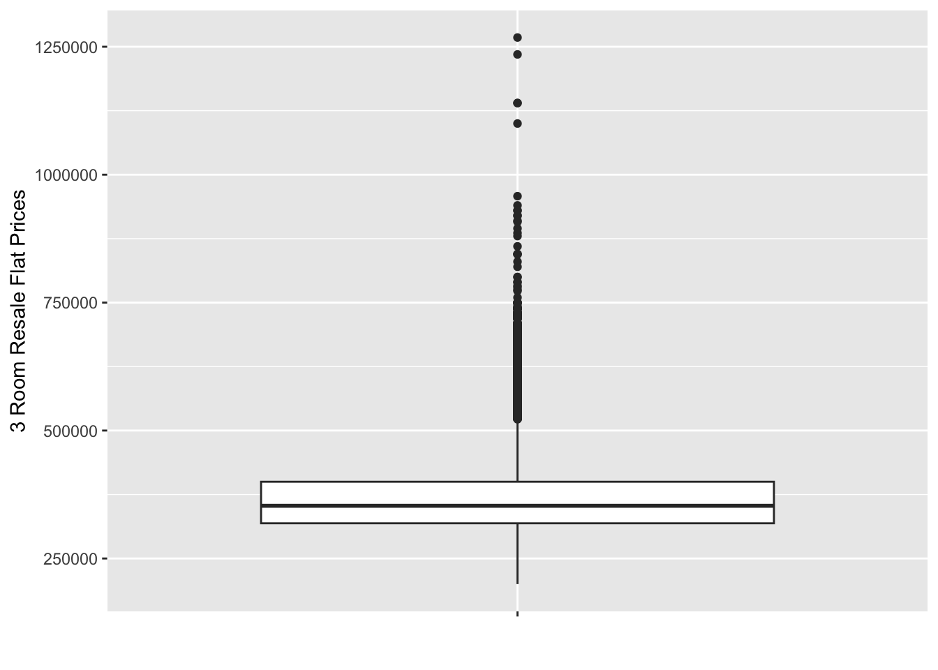
ggplot(data=four_room_2021_22_sf, aes(x=`resale_price`)) +
geom_histogram(bins=20, color="black", fill="pink") +
labs(title = "Distribution of Resale Prices for 3 Room Flats (2021 - 2022)",
x = "Resale Prices",
y = 'Frequency') +
scale_x_continuous(labels = scales::comma) +
scale_y_continuous(labels = scales::comma)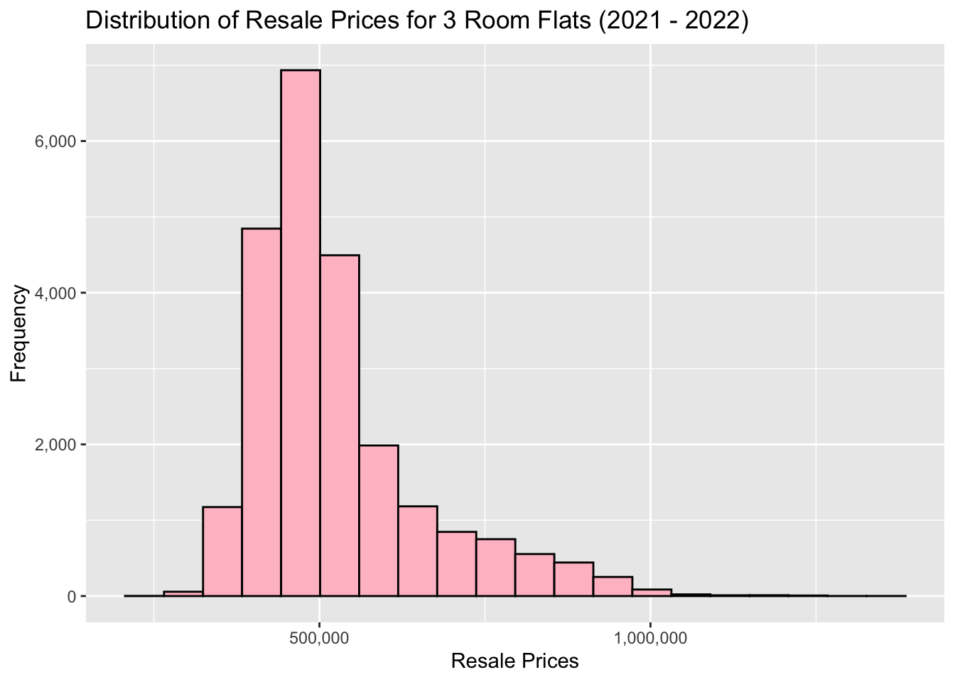
ggplot(data = four_room_2021_22_sf, aes(x = '', y = resale_price)) +
geom_boxplot() +
labs(x='', y='3 Room Resale Flat Prices')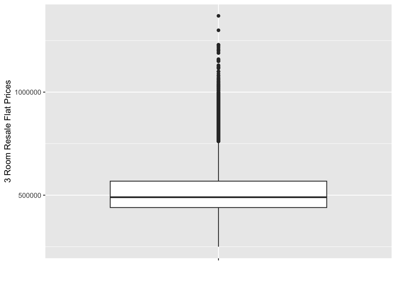
ggplot(data=five_room_2021_22_sf, aes(x=`resale_price`)) +
geom_histogram(bins=20, color="black", fill="pink") +
labs(title = "Distribution of Resale Prices for 3 Room Flats (2021 - 2022)",
x = "Resale Prices",
y = 'Frequency') +
scale_x_continuous(labels = scales::comma) +
scale_y_continuous(labels = scales::comma)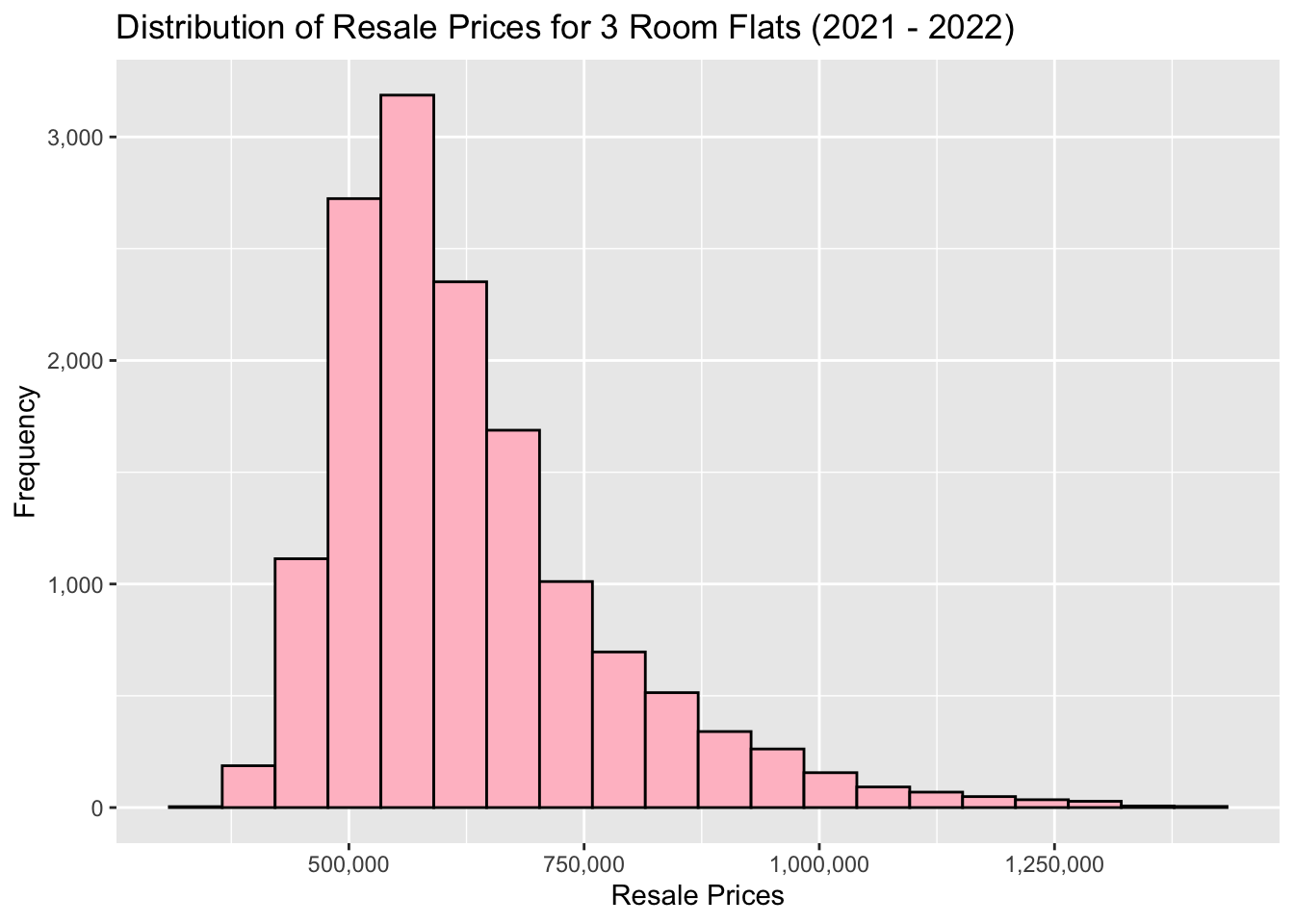
ggplot(data = five_room_2021_22_sf, aes(x = '', y = resale_price)) +
geom_boxplot() +
labs(x='', y='3 Room Resale Flat Prices')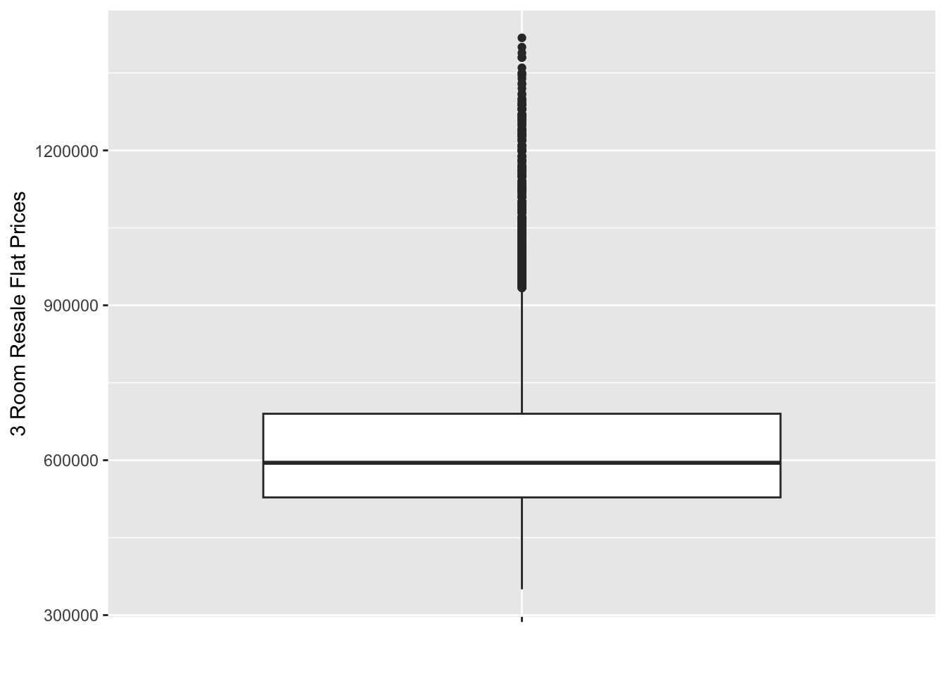
As we can see, all 3 have an distinct right skew. This indicates that more resale flats were bought at relatively lower price.
From both our histograms and boxplots, we can also see the mode of the data increasing gradually as we move from 3 to 4 to 5 rooms. This aligns with out expectations, as a flat with more rooms should on average cost more than one with fewer.
Although we do see quite a lot of outliers in our boxplots (with the highest prices being well over 2-3 times the mean price), in general we see that 3 room flats being in about the 300k - 400k range, 4 room flats being in the 450k-550k range, and 5 rooms flats in the 500k-700k range.
Flat Factors
Let us look at the distribution of our Resale Flat factors, namely floor_area_sqm, storey_range, remaining_lease and age_of_unit.
floor_area_plot <- ggplot(data = three_room_2021_22_sf, aes(x = `floor_area_sqm`)) +
geom_histogram(bins=20, color="black", fill = 'pink')
storey_range_plot <- ggplot(data = three_room_2021_22_sf, aes(x = `storey_range`)) +
geom_histogram(bins=20, color="black", fill = 'pink')
remaining_lease_plot <- ggplot(data = three_room_2021_22_sf, aes(x = `remaining_lease`)) +
geom_histogram(bins=20, color="black", fill = 'pink')
unit_age_plot <- ggplot(data = three_room_2021_22_sf, aes(x = `age_of_unit`)) +
geom_histogram(bins=20, color="black", fill = 'pink')
ggarrange(floor_area_plot, storey_range_plot, remaining_lease_plot, unit_age_plot, ncol = 2, nrow = 2)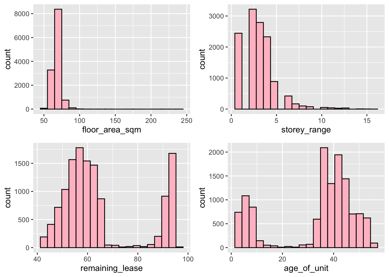
floor_area_plot <- ggplot(data = four_room_2021_22_sf, aes(x = `floor_area_sqm`)) +
geom_histogram(bins=20, color="black", fill = 'pink')
storey_range_plot <- ggplot(data = four_room_2021_22_sf, aes(x = `storey_range`)) +
geom_histogram(bins=20, color="black", fill = 'pink')
remaining_lease_plot <- ggplot(data = four_room_2021_22_sf, aes(x = `remaining_lease`)) +
geom_histogram(bins=20, color="black", fill = 'pink')
unit_age_plot <- ggplot(data = four_room_2021_22_sf, aes(x = `age_of_unit`)) +
geom_histogram(bins=20, color="black", fill = 'pink')
ggarrange(floor_area_plot, storey_range_plot, remaining_lease_plot, unit_age_plot, ncol = 2, nrow = 2)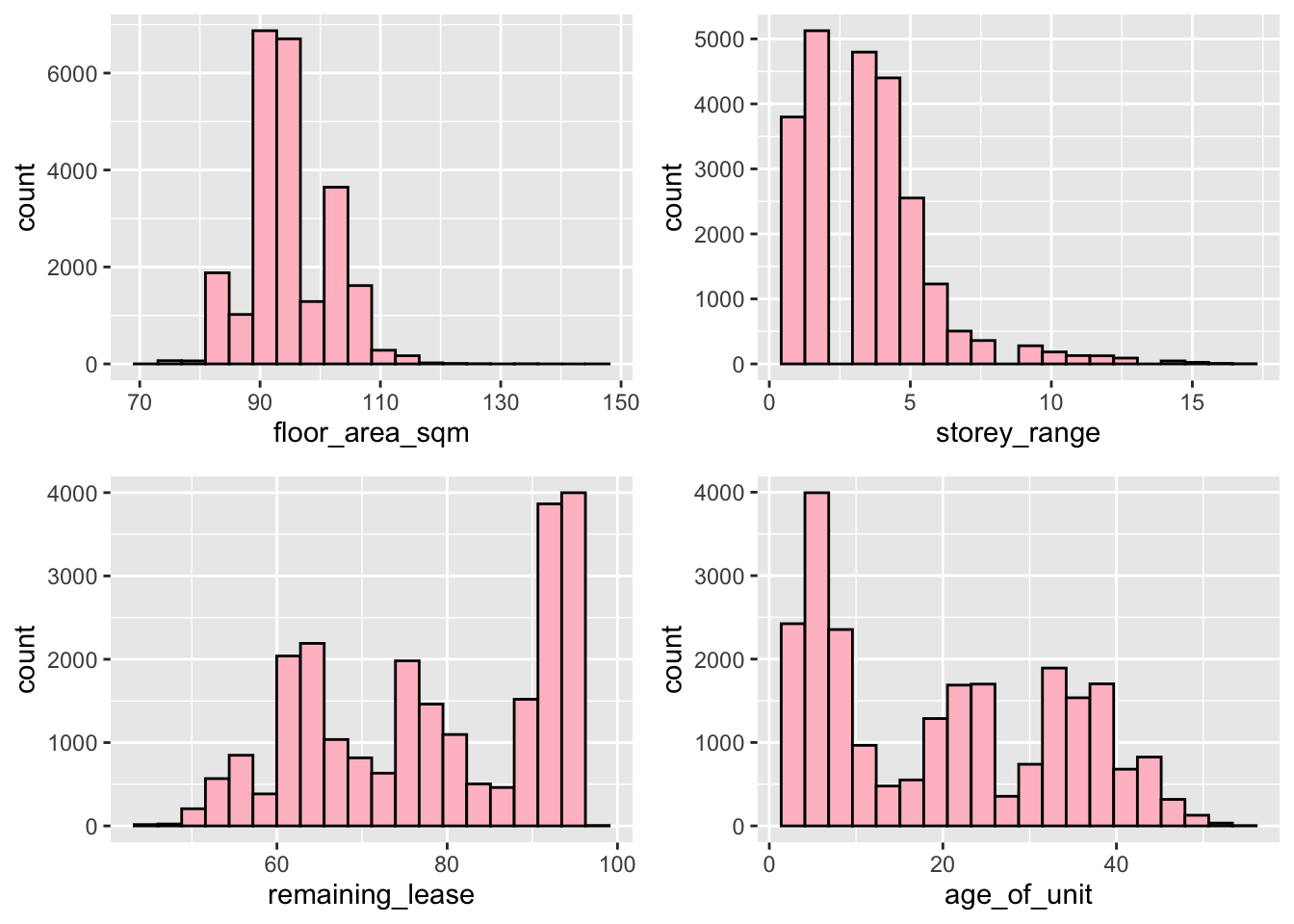
floor_area_plot <- ggplot(data = five_room_2021_22_sf, aes(x = `floor_area_sqm`)) +
geom_histogram(bins=20, color="black", fill = 'pink')
storey_range_plot <- ggplot(data = five_room_2021_22_sf, aes(x = `storey_range`)) +
geom_histogram(bins=20, color="black", fill = 'pink')
remaining_lease_plot <- ggplot(data = five_room_2021_22_sf, aes(x = `remaining_lease`)) +
geom_histogram(bins=20, color="black", fill = 'pink')
unit_age_plot <- ggplot(data = five_room_2021_22_sf, aes(x = `age_of_unit`)) +
geom_histogram(bins=20, color="black", fill = 'pink')
ggarrange(floor_area_plot, storey_range_plot, remaining_lease_plot, unit_age_plot, ncol = 2, nrow = 2)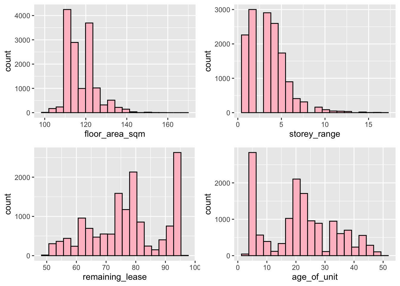
Locational Factors
And lastly, we can visualise our locational factors; PROX_CBD, PROX_ELDERCARE, PROX_HAWKER_CENTRE, PROX_MRT, PROX_PARK, PROX_GOOD_PRI_SCH, PROX_MALL, PROX_SUPERMARKET, NUM_KINDERGARTEN, NUM_CHILDCARE, NUM_BUS_STOP and NUM_PRI_SCH.
PROX_CBD_plot <- ggplot(data = three_room_2021_22_sf, aes(x = `PROX_CBD`)) +
geom_histogram(bins=20, color="black", fill = 'pink')
PROX_ELDERCARE_plot <- ggplot(data = three_room_2021_22_sf, aes(x = `PROX_ELDERCARE`)) +
geom_histogram(bins=20, color="black", fill = 'pink')
PROX_HAWKER_CENTRE_plot <- ggplot(data = three_room_2021_22_sf,
aes(x = `PROX_HAWKER_CENTRE`)) +
geom_histogram(bins=20, color="black", fill = 'pink')
PROX_MRT_plot <- ggplot(data = three_room_2021_22_sf, aes(x = `PROX_MRT`)) +
geom_histogram(bins=20, color="black", fill = 'pink')
PROX_PARK_plot <- ggplot(data = three_room_2021_22_sf, aes(x = `PROX_PARK`)) +
geom_histogram(bins=20, color="black", fill = 'pink')
PROX_GOOD_PRI_SCH_plot <- ggplot(data = three_room_2021_22_sf,
aes(x = `PROX_GOOD_PRI_SCH`)) +
geom_histogram(bins=20, color="black", fill = 'pink')
PROX_MALL_plot <- ggplot(data = three_room_2021_22_sf,
aes(x = `PROX_MALL`)) +
geom_histogram(bins=20, color="black", fill = 'pink')
PROX_SUPERMARKET_plot <- ggplot(data = three_room_2021_22_sf,
aes(x = `PROX_SUPERMARKET`)) +
geom_histogram(bins=20, color="black", fill = 'pink')
NUM_KINDERGARTEN_plot <- ggplot(data = three_room_2021_22_sf,
aes(x = `NUM_KINDERGARTEN`)) +
geom_histogram(bins=20, color="black", fill = 'pink')
NUM_CHILDCARE_plot <- ggplot(data = three_room_2021_22_sf, aes(x = `NUM_CHILDCARE`)) +
geom_histogram(bins=20, color="black", fill = 'pink')
NUM_BUS_STOP_plot <- ggplot(data = three_room_2021_22_sf, aes(x = `NUM_BUS_STOP`)) +
geom_histogram(bins=20, color="black", fill = 'pink')
NUM_PRI_SCH_plot <- ggplot(data = three_room_2021_22_sf, aes(x = `NUM_PRI_SCH`)) +
geom_histogram(bins=20, color="black", fill = 'pink')
ggarrange(PROX_CBD_plot, PROX_ELDERCARE_plot, PROX_HAWKER_CENTRE_plot, PROX_MRT_plot,
PROX_PARK_plot, PROX_GOOD_PRI_SCH_plot, PROX_MALL_plot,
PROX_SUPERMARKET_plot, NUM_KINDERGARTEN_plot, NUM_CHILDCARE_plot,
NUM_BUS_STOP_plot, NUM_PRI_SCH_plot, ncol = 3, nrow = 4)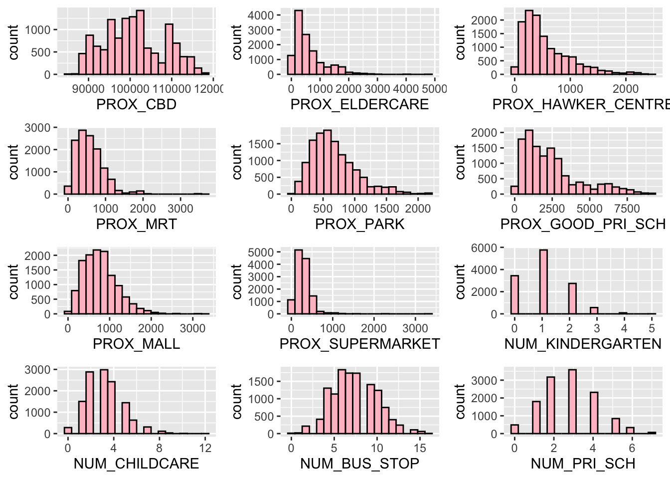
PROX_CBD_plot <- ggplot(data = four_room_2021_22_sf, aes(x = `PROX_CBD`)) +
geom_histogram(bins=20, color="black", fill = 'pink')
PROX_ELDERCARE_plot <- ggplot(data = four_room_2021_22_sf, aes(x = `PROX_ELDERCARE`)) +
geom_histogram(bins=20, color="black", fill = 'pink')
PROX_HAWKER_CENTRE_plot <- ggplot(data = four_room_2021_22_sf,
aes(x = `PROX_HAWKER_CENTRE`)) +
geom_histogram(bins=20, color="black", fill = 'pink')
PROX_MRT_plot <- ggplot(data = four_room_2021_22_sf, aes(x = `PROX_MRT`)) +
geom_histogram(bins=20, color="black", fill = 'pink')
PROX_PARK_plot <- ggplot(data = four_room_2021_22_sf, aes(x = `PROX_PARK`)) +
geom_histogram(bins=20, color="black", fill = 'pink')
PROX_GOOD_PRI_SCH_plot <- ggplot(data = four_room_2021_22_sf,
aes(x = `PROX_GOOD_PRI_SCH`)) +
geom_histogram(bins=20, color="black", fill = 'pink')
PROX_MALL_plot <- ggplot(data = four_room_2021_22_sf,
aes(x = `PROX_MALL`)) +
geom_histogram(bins=20, color="black", fill = 'pink')
PROX_SUPERMARKET_plot <- ggplot(data = four_room_2021_22_sf,
aes(x = `PROX_SUPERMARKET`)) +
geom_histogram(bins=20, color="black", fill = 'pink')
NUM_KINDERGARTEN_plot <- ggplot(data = four_room_2021_22_sf,
aes(x = `NUM_KINDERGARTEN`)) +
geom_histogram(bins=20, color="black", fill = 'pink')
NUM_CHILDCARE_plot <- ggplot(data = four_room_2021_22_sf, aes(x = `NUM_CHILDCARE`)) +
geom_histogram(bins=20, color="black", fill = 'pink')
NUM_BUS_STOP_plot <- ggplot(data = four_room_2021_22_sf, aes(x = `NUM_BUS_STOP`)) +
geom_histogram(bins=20, color="black", fill = 'pink')
NUM_PRI_SCH_plot <- ggplot(data = four_room_2021_22_sf, aes(x = `NUM_PRI_SCH`)) +
geom_histogram(bins=20, color="black", fill = 'pink')
ggarrange(PROX_CBD_plot, PROX_ELDERCARE_plot, PROX_HAWKER_CENTRE_plot, PROX_MRT_plot,
PROX_PARK_plot, PROX_GOOD_PRI_SCH_plot, PROX_MALL_plot,
PROX_SUPERMARKET_plot, NUM_KINDERGARTEN_plot, NUM_CHILDCARE_plot,
NUM_BUS_STOP_plot, NUM_PRI_SCH_plot, ncol = 3, nrow = 4)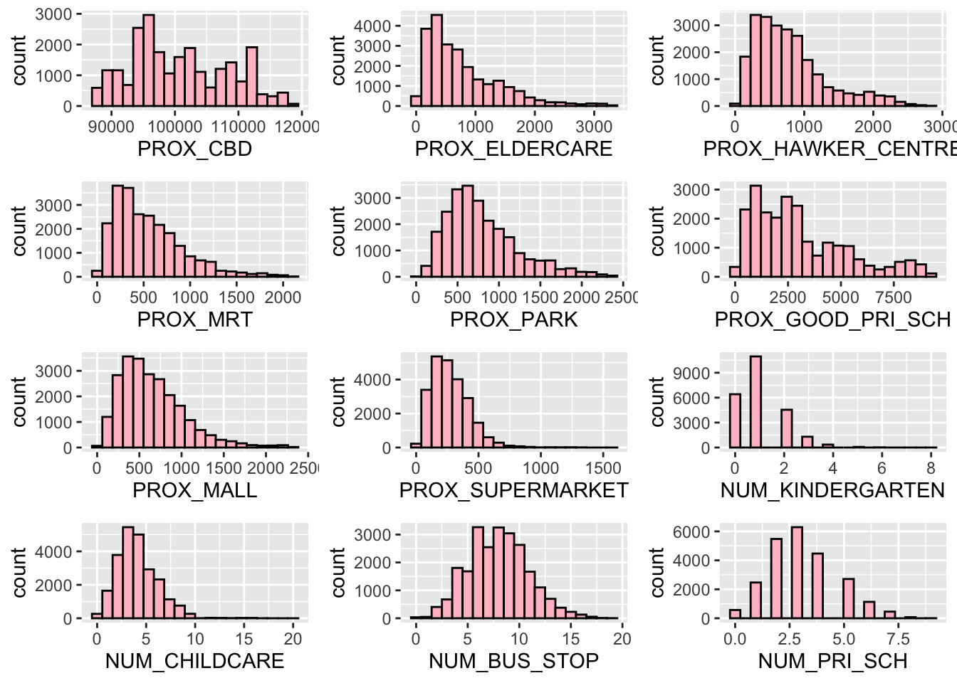
PROX_CBD_plot <- ggplot(data = five_room_2021_22_sf, aes(x = `PROX_CBD`)) +
geom_histogram(bins=20, color="black", fill = 'pink')
PROX_ELDERCARE_plot <- ggplot(data = five_room_2021_22_sf, aes(x = `PROX_ELDERCARE`)) +
geom_histogram(bins=20, color="black", fill = 'pink')
PROX_HAWKER_CENTRE_plot <- ggplot(data = five_room_2021_22_sf,
aes(x = `PROX_HAWKER_CENTRE`)) +
geom_histogram(bins=20, color="black", fill = 'pink')
PROX_MRT_plot <- ggplot(data = five_room_2021_22_sf, aes(x = `PROX_MRT`)) +
geom_histogram(bins=20, color="black", fill = 'pink')
PROX_PARK_plot <- ggplot(data = five_room_2021_22_sf, aes(x = `PROX_PARK`)) +
geom_histogram(bins=20, color="black", fill = 'pink')
PROX_GOOD_PRI_SCH_plot <- ggplot(data = five_room_2021_22_sf,
aes(x = `PROX_GOOD_PRI_SCH`)) +
geom_histogram(bins=20, color="black", fill = 'pink')
PROX_MALL_plot <- ggplot(data = five_room_2021_22_sf,
aes(x = `PROX_MALL`)) +
geom_histogram(bins=20, color="black", fill = 'pink')
PROX_SUPERMARKET_plot <- ggplot(data = five_room_2021_22_sf,
aes(x = `PROX_SUPERMARKET`)) +
geom_histogram(bins=20, color="black", fill = 'pink')
NUM_KINDERGARTEN_plot <- ggplot(data = five_room_2021_22_sf,
aes(x = `NUM_KINDERGARTEN`)) +
geom_histogram(bins=20, color="black", fill = 'pink')
NUM_CHILDCARE_plot <- ggplot(data = five_room_2021_22_sf, aes(x = `NUM_CHILDCARE`)) +
geom_histogram(bins=20, color="black", fill = 'pink')
NUM_BUS_STOP_plot <- ggplot(data = five_room_2021_22_sf, aes(x = `NUM_BUS_STOP`)) +
geom_histogram(bins=20, color="black", fill = 'pink')
NUM_PRI_SCH_plot <- ggplot(data = five_room_2021_22_sf, aes(x = `NUM_PRI_SCH`)) +
geom_histogram(bins=20, color="black", fill = 'pink')
ggarrange(PROX_CBD_plot, PROX_ELDERCARE_plot, PROX_HAWKER_CENTRE_plot, PROX_MRT_plot,
PROX_PARK_plot, PROX_GOOD_PRI_SCH_plot, PROX_MALL_plot,
PROX_SUPERMARKET_plot, NUM_KINDERGARTEN_plot, NUM_CHILDCARE_plot,
NUM_BUS_STOP_plot, NUM_PRI_SCH_plot, ncol = 3, nrow = 4)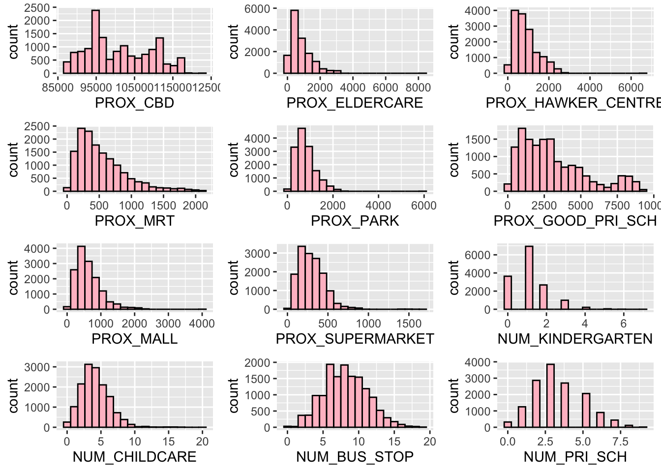
Spatial Visualisation
Let us quickly revisit the spatial visualisation of our resale price data.
tmap_mode("view")
tm_shape(mpsz) +
tm_polygons() +
tm_shape(three_room_2021_22_sf)+
tm_dots(col = "resale_price",
size = 0.01,
border.col = "black",
border.lwd = 0.5) +
tmap_options(check.and.fix = TRUE) +
tm_view(set.zoom.limits = c(11, 16))tmap_mode("view")
tm_shape(mpsz) +
tm_polygons() +
tm_shape(four_room_2021_22_sf)+
tm_dots(col = "resale_price",
size = 0.01,
border.col = "black",
border.lwd = 0.5) +
tmap_options(check.and.fix = TRUE) +
tm_view(set.zoom.limits = c(11, 16))