pacman::p_load(olsrr, corrplot, ggpubr, sf, spdep, GWmodel, tmap, tidyverse, gtsummary)
# OR load corrplot via tools tab
# pacman::p_load(olsrr, ggpubr, sf, spdep, GWmodel, tmap, tidyverse, gtsummary)In-Class Exercise 8: Geographically Weighted Regression
Imports
Import Packages
Geospatial Data Import & Pre-Processing
mpsz = st_read(dsn = "data/geospatial", layer = "MP14_SUBZONE_WEB_PL")Reading layer `MP14_SUBZONE_WEB_PL' from data source
`/Users/michelle/Desktop/IS415/shelle-mim/IS415-GAA/Hands-on_Exercise/Wk9/data/geospatial'
using driver `ESRI Shapefile'
Simple feature collection with 323 features and 15 fields
Geometry type: MULTIPOLYGON
Dimension: XY
Bounding box: xmin: 2667.538 ymin: 15748.72 xmax: 56396.44 ymax: 50256.33
Projected CRS: SVY21mpsz_svy21 <- st_transform(mpsz, 3414)st_crs(mpsz_svy21)Coordinate Reference System:
User input: EPSG:3414
wkt:
PROJCRS["SVY21 / Singapore TM",
BASEGEOGCRS["SVY21",
DATUM["SVY21",
ELLIPSOID["WGS 84",6378137,298.257223563,
LENGTHUNIT["metre",1]]],
PRIMEM["Greenwich",0,
ANGLEUNIT["degree",0.0174532925199433]],
ID["EPSG",4757]],
CONVERSION["Singapore Transverse Mercator",
METHOD["Transverse Mercator",
ID["EPSG",9807]],
PARAMETER["Latitude of natural origin",1.36666666666667,
ANGLEUNIT["degree",0.0174532925199433],
ID["EPSG",8801]],
PARAMETER["Longitude of natural origin",103.833333333333,
ANGLEUNIT["degree",0.0174532925199433],
ID["EPSG",8802]],
PARAMETER["Scale factor at natural origin",1,
SCALEUNIT["unity",1],
ID["EPSG",8805]],
PARAMETER["False easting",28001.642,
LENGTHUNIT["metre",1],
ID["EPSG",8806]],
PARAMETER["False northing",38744.572,
LENGTHUNIT["metre",1],
ID["EPSG",8807]]],
CS[Cartesian,2],
AXIS["northing (N)",north,
ORDER[1],
LENGTHUNIT["metre",1]],
AXIS["easting (E)",east,
ORDER[2],
LENGTHUNIT["metre",1]],
USAGE[
SCOPE["Cadastre, engineering survey, topographic mapping."],
AREA["Singapore - onshore and offshore."],
BBOX[1.13,103.59,1.47,104.07]],
ID["EPSG",3414]]# View extent
st_bbox(mpsz_svy21) xmin ymin xmax ymax
2667.538 15748.721 56396.440 50256.334 Aspatial Data Import & Pre-Processing
condo_resale = read_csv("data/aspatial/Condo_resale_2015.csv")summary(condo_resale) LATITUDE LONGITUDE POSTCODE SELLING_PRICE
Min. :1.240 Min. :103.7 Min. : 18965 Min. : 540000
1st Qu.:1.309 1st Qu.:103.8 1st Qu.:259849 1st Qu.: 1100000
Median :1.328 Median :103.8 Median :469298 Median : 1383222
Mean :1.334 Mean :103.8 Mean :440439 Mean : 1751211
3rd Qu.:1.357 3rd Qu.:103.9 3rd Qu.:589486 3rd Qu.: 1950000
Max. :1.454 Max. :104.0 Max. :828833 Max. :18000000
AREA_SQM AGE PROX_CBD PROX_CHILDCARE
Min. : 34.0 Min. : 0.00 Min. : 0.3869 Min. :0.004927
1st Qu.:103.0 1st Qu.: 5.00 1st Qu.: 5.5574 1st Qu.:0.174481
Median :121.0 Median :11.00 Median : 9.3567 Median :0.258135
Mean :136.5 Mean :12.14 Mean : 9.3254 Mean :0.326313
3rd Qu.:156.0 3rd Qu.:18.00 3rd Qu.:12.6661 3rd Qu.:0.368293
Max. :619.0 Max. :37.00 Max. :19.1804 Max. :3.465726
PROX_ELDERLYCARE PROX_URA_GROWTH_AREA PROX_HAWKER_MARKET PROX_KINDERGARTEN
Min. :0.05451 Min. :0.2145 Min. :0.05182 Min. :0.004927
1st Qu.:0.61254 1st Qu.:3.1643 1st Qu.:0.55245 1st Qu.:0.276345
Median :0.94179 Median :4.6186 Median :0.90842 Median :0.413385
Mean :1.05351 Mean :4.5981 Mean :1.27987 Mean :0.458903
3rd Qu.:1.35122 3rd Qu.:5.7550 3rd Qu.:1.68578 3rd Qu.:0.578474
Max. :3.94916 Max. :9.1554 Max. :5.37435 Max. :2.229045
PROX_MRT PROX_PARK PROX_PRIMARY_SCH PROX_TOP_PRIMARY_SCH
Min. :0.05278 Min. :0.02906 Min. :0.07711 Min. :0.07711
1st Qu.:0.34646 1st Qu.:0.26211 1st Qu.:0.44024 1st Qu.:1.34451
Median :0.57430 Median :0.39926 Median :0.63505 Median :1.88213
Mean :0.67316 Mean :0.49802 Mean :0.75471 Mean :2.27347
3rd Qu.:0.84844 3rd Qu.:0.65592 3rd Qu.:0.95104 3rd Qu.:2.90954
Max. :3.48037 Max. :2.16105 Max. :3.92899 Max. :6.74819
PROX_SHOPPING_MALL PROX_SUPERMARKET PROX_BUS_STOP NO_Of_UNITS
Min. :0.0000 Min. :0.0000 Min. :0.001595 Min. : 18.0
1st Qu.:0.5258 1st Qu.:0.3695 1st Qu.:0.098356 1st Qu.: 188.8
Median :0.9357 Median :0.5687 Median :0.151710 Median : 360.0
Mean :1.0455 Mean :0.6141 Mean :0.193974 Mean : 409.2
3rd Qu.:1.3994 3rd Qu.:0.7862 3rd Qu.:0.220466 3rd Qu.: 590.0
Max. :3.4774 Max. :2.2441 Max. :2.476639 Max. :1703.0
FAMILY_FRIENDLY FREEHOLD LEASEHOLD_99YR
Min. :0.0000 Min. :0.0000 Min. :0.0000
1st Qu.:0.0000 1st Qu.:0.0000 1st Qu.:0.0000
Median :0.0000 Median :0.0000 Median :0.0000
Mean :0.4868 Mean :0.4227 Mean :0.4882
3rd Qu.:1.0000 3rd Qu.:1.0000 3rd Qu.:1.0000
Max. :1.0000 Max. :1.0000 Max. :1.0000 # Make sure that in the summary statistics theres no an excessive number of 0 / if data has a good spreadcondo_resale.sf <- st_as_sf(condo_resale,
coords = c("LONGITUDE", "LATITUDE"),
crs=4326) %>%
st_transform(crs=3414)head(condo_resale.sf)Simple feature collection with 6 features and 21 fields
Geometry type: POINT
Dimension: XY
Bounding box: xmin: 22085.12 ymin: 29951.54 xmax: 41042.56 ymax: 34546.2
Projected CRS: SVY21 / Singapore TM
# A tibble: 6 × 22
POSTCODE SELLI…¹ AREA_…² AGE PROX_…³ PROX_…⁴ PROX_…⁵ PROX_…⁶ PROX_…⁷ PROX_…⁸
<dbl> <dbl> <dbl> <dbl> <dbl> <dbl> <dbl> <dbl> <dbl> <dbl>
1 118635 3000000 309 30 7.94 0.166 2.52 6.62 1.77 0.0584
2 288420 3880000 290 32 6.61 0.280 1.93 7.51 0.545 0.616
3 267833 3325000 248 33 6.90 0.429 0.502 6.46 0.378 0.141
4 258380 4250000 127 7 4.04 0.395 1.99 4.91 1.68 0.382
5 467169 1400000 145 28 11.8 0.119 1.12 6.41 0.565 0.461
6 466472 1320000 139 22 10.3 0.125 0.789 5.09 0.781 0.0994
# … with 12 more variables: PROX_MRT <dbl>, PROX_PARK <dbl>,
# PROX_PRIMARY_SCH <dbl>, PROX_TOP_PRIMARY_SCH <dbl>,
# PROX_SHOPPING_MALL <dbl>, PROX_SUPERMARKET <dbl>, PROX_BUS_STOP <dbl>,
# NO_Of_UNITS <dbl>, FAMILY_FRIENDLY <dbl>, FREEHOLD <dbl>,
# LEASEHOLD_99YR <dbl>, geometry <POINT [m]>, and abbreviated variable names
# ¹SELLING_PRICE, ²AREA_SQM, ³PROX_CBD, ⁴PROX_CHILDCARE, ⁵PROX_ELDERLYCARE,
# ⁶PROX_URA_GROWTH_AREA, ⁷PROX_HAWKER_MARKET, ⁸PROX_KINDERGARTENExploratory Data Analysis
Statistical Graphics
# Look at selling price distribution
ggplot(data=condo_resale.sf, aes(x=`SELLING_PRICE`)) +
geom_histogram(bins=20, color="black", fill="light blue")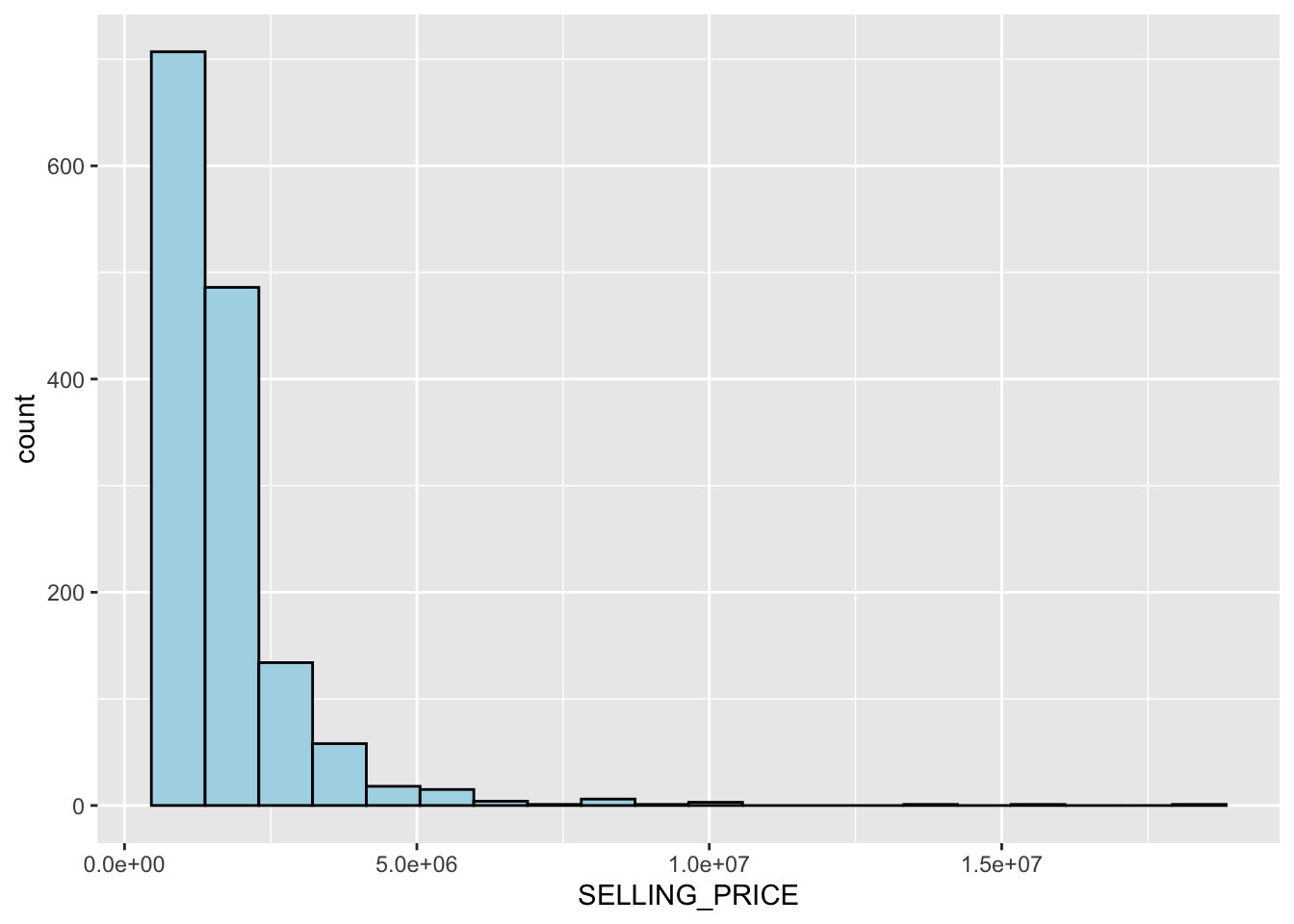
# Get log selling price
condo_resale.sf <- condo_resale.sf %>%
mutate(`LOG_SELLING_PRICE` = log(SELLING_PRICE))
# Plot
ggplot(data=condo_resale.sf, aes(x=`LOG_SELLING_PRICE`)) +
geom_histogram(bins=20, color="black", fill="light blue")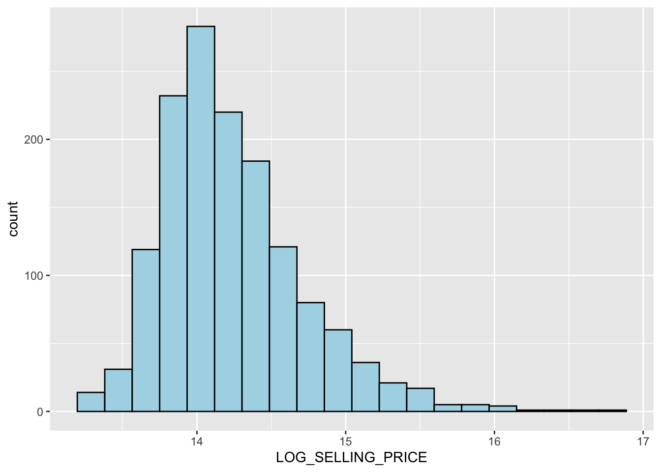
AREA_SQM <- ggplot(data=condo_resale.sf, aes(x= `AREA_SQM`)) +
geom_histogram(bins=20, color="black", fill="light blue")
AGE <- ggplot(data=condo_resale.sf, aes(x= `AGE`)) +
geom_histogram(bins=20, color="black", fill="light blue")
PROX_CBD <- ggplot(data=condo_resale.sf, aes(x= `PROX_CBD`)) +
geom_histogram(bins=20, color="black", fill="light blue")
PROX_CHILDCARE <- ggplot(data=condo_resale.sf, aes(x= `PROX_CHILDCARE`)) +
geom_histogram(bins=20, color="black", fill="light blue")
PROX_ELDERLYCARE <- ggplot(data=condo_resale.sf, aes(x= `PROX_ELDERLYCARE`)) +
geom_histogram(bins=20, color="black", fill="light blue")
PROX_URA_GROWTH_AREA <- ggplot(data=condo_resale.sf,
aes(x= `PROX_URA_GROWTH_AREA`)) +
geom_histogram(bins=20, color="black", fill="light blue")
PROX_HAWKER_MARKET <- ggplot(data=condo_resale.sf, aes(x= `PROX_HAWKER_MARKET`)) +
geom_histogram(bins=20, color="black", fill="light blue")
PROX_KINDERGARTEN <- ggplot(data=condo_resale.sf, aes(x= `PROX_KINDERGARTEN`)) +
geom_histogram(bins=20, color="black", fill="light blue")
PROX_MRT <- ggplot(data=condo_resale.sf, aes(x= `PROX_MRT`)) +
geom_histogram(bins=20, color="black", fill="light blue")
PROX_PARK <- ggplot(data=condo_resale.sf, aes(x= `PROX_PARK`)) +
geom_histogram(bins=20, color="black", fill="light blue")
PROX_PRIMARY_SCH <- ggplot(data=condo_resale.sf, aes(x= `PROX_PRIMARY_SCH`)) +
geom_histogram(bins=20, color="black", fill="light blue")
PROX_TOP_PRIMARY_SCH <- ggplot(data=condo_resale.sf,
aes(x= `PROX_TOP_PRIMARY_SCH`)) +
geom_histogram(bins=20, color="black", fill="light blue")
ggarrange(AREA_SQM, AGE, PROX_CBD, PROX_CHILDCARE, PROX_ELDERLYCARE,
PROX_URA_GROWTH_AREA, PROX_HAWKER_MARKET, PROX_KINDERGARTEN, PROX_MRT,
PROX_PARK, PROX_PRIMARY_SCH, PROX_TOP_PRIMARY_SCH,
ncol = 3, nrow = 4)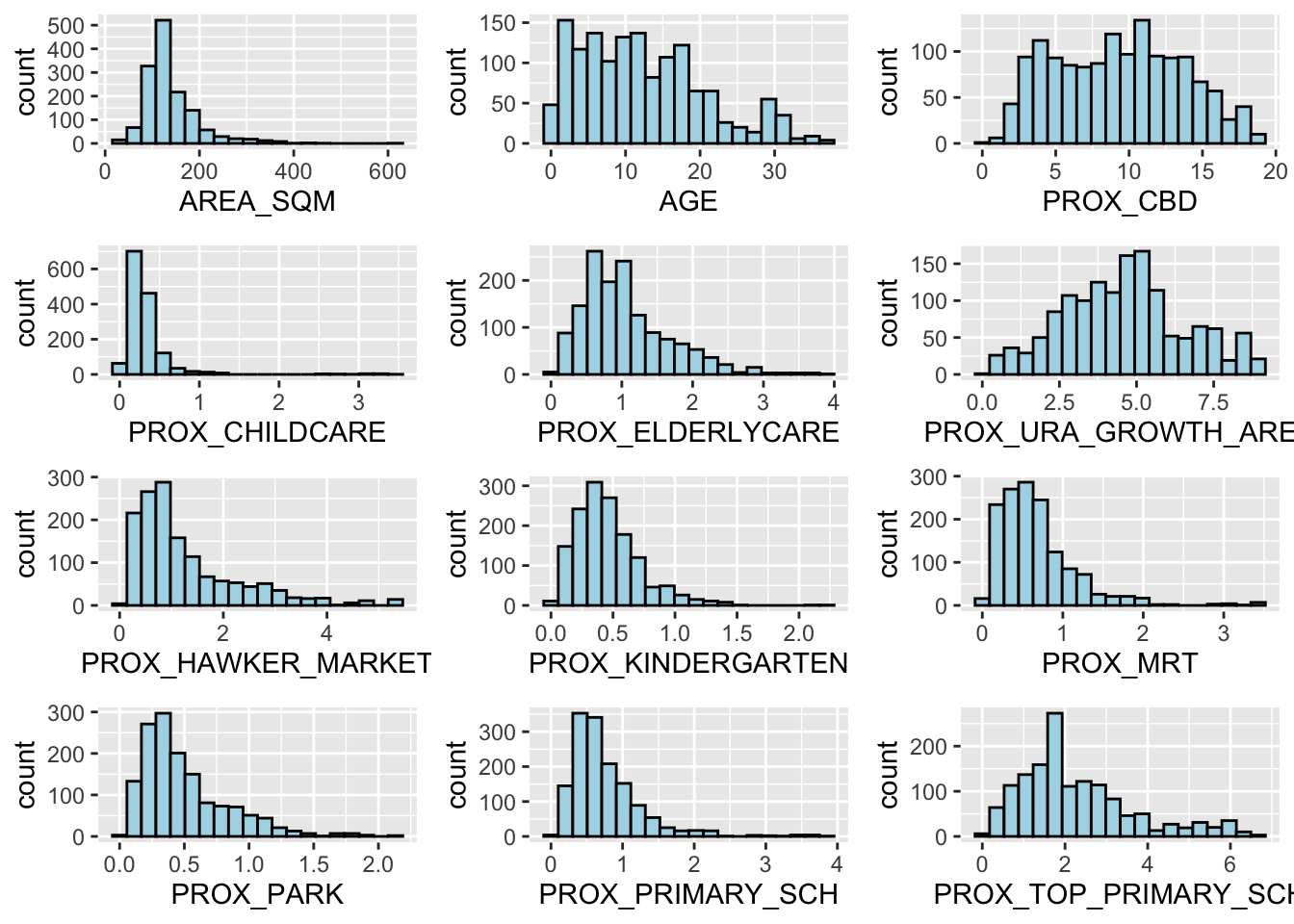
Statistical Point Map
tmap_mode("view")
tm_shape(mpsz_svy21)+
tm_polygons() +
tm_shape(condo_resale.sf) +
tm_dots(col = "SELLING_PRICE",
alpha = 0.6,
style="quantile") +
tm_view(set.zoom.limits = c(11,14)) +
tmap_options(check.and.fix = TRUE)tmap_mode("plot")Hedonic Pricing Modelling
Simple Linear Regression Method
condo.slr <- lm(formula=SELLING_PRICE ~ AREA_SQM, data = condo_resale.sf)
summary(condo.slr)
Call:
lm(formula = SELLING_PRICE ~ AREA_SQM, data = condo_resale.sf)
Residuals:
Min 1Q Median 3Q Max
-3695815 -391764 -87517 258900 13503875
Coefficients:
Estimate Std. Error t value Pr(>|t|)
(Intercept) -258121.1 63517.2 -4.064 5.09e-05 ***
AREA_SQM 14719.0 428.1 34.381 < 2e-16 ***
---
Signif. codes: 0 '***' 0.001 '**' 0.01 '*' 0.05 '.' 0.1 ' ' 1
Residual standard error: 942700 on 1434 degrees of freedom
Multiple R-squared: 0.4518, Adjusted R-squared: 0.4515
F-statistic: 1182 on 1 and 1434 DF, p-value: < 2.2e-16ggplot(data=condo_resale.sf,
aes(x=`AREA_SQM`, y=`SELLING_PRICE`)) +
geom_point() +
geom_smooth(method = lm)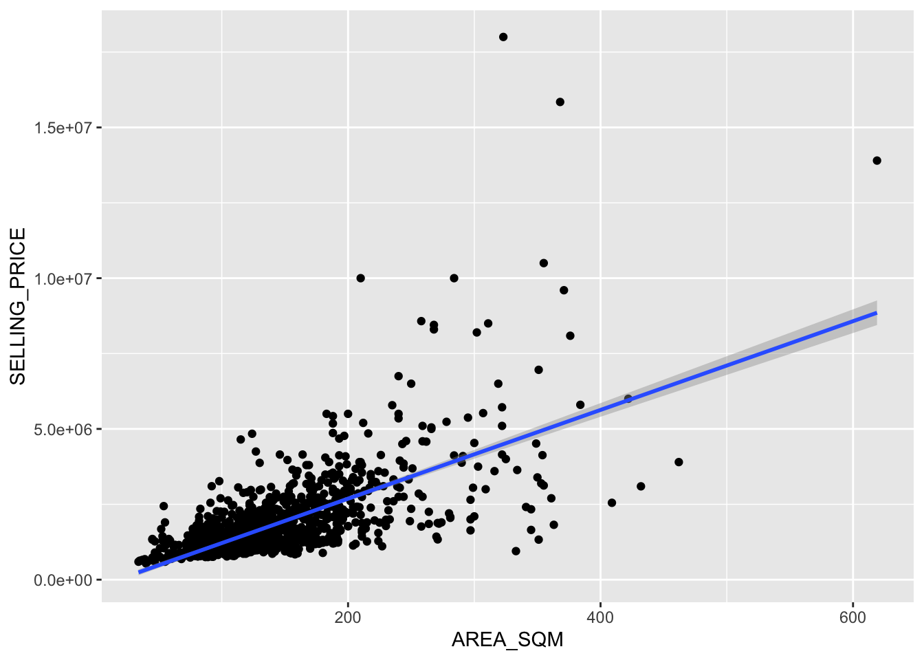
Multiple Linear Regression Method
# Can easily eyeball the dark red and dark blue colors and determine these are the ones that are highly correlated
corrplot(cor(condo_resale[, 5:23]), diag = FALSE, order = "AOE",
tl.pos = "td", tl.cex = 0.5, method = "number", type = "upper")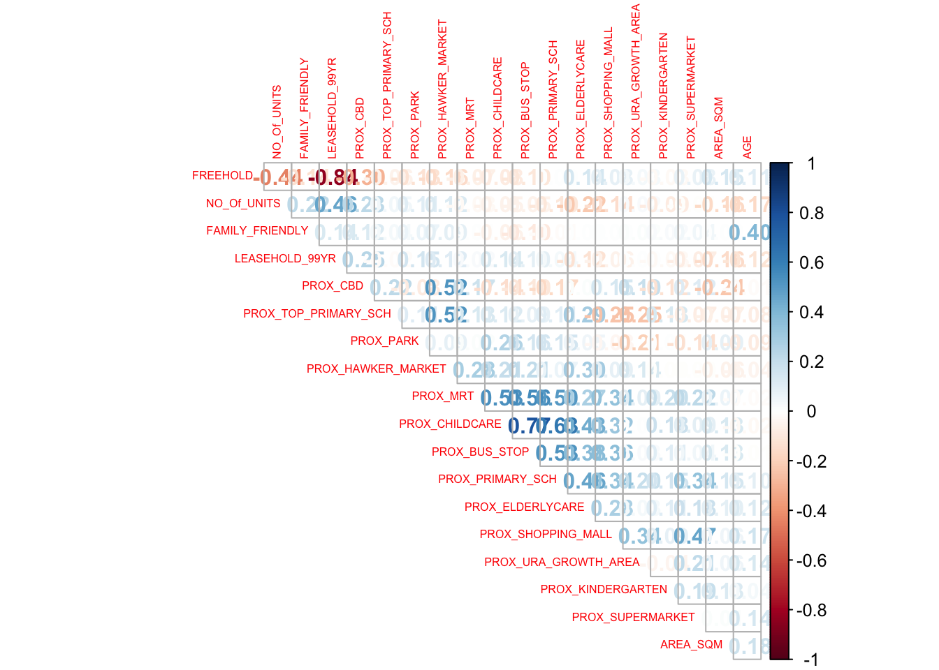
Building a hedonic pricing model using multiple linear regression method
Calibrate regression model
Will be using LM -> is from base R, allows you to do generic linear regression
There is also GLM which has more types of models
# Calibrate regression model
# Indep var Follow by dep vars
condo.mlr <- lm(formula = SELLING_PRICE ~ AREA_SQM + AGE +
PROX_CBD + PROX_CHILDCARE + PROX_ELDERLYCARE +
PROX_URA_GROWTH_AREA + PROX_HAWKER_MARKET + PROX_KINDERGARTEN +
PROX_MRT + PROX_PARK + PROX_PRIMARY_SCH +
PROX_TOP_PRIMARY_SCH + PROX_SHOPPING_MALL + PROX_SUPERMARKET +
PROX_BUS_STOP + NO_Of_UNITS + FAMILY_FRIENDLY + FREEHOLD,
data=condo_resale.sf)
summary(condo.mlr)
Call:
lm(formula = SELLING_PRICE ~ AREA_SQM + AGE + PROX_CBD + PROX_CHILDCARE +
PROX_ELDERLYCARE + PROX_URA_GROWTH_AREA + PROX_HAWKER_MARKET +
PROX_KINDERGARTEN + PROX_MRT + PROX_PARK + PROX_PRIMARY_SCH +
PROX_TOP_PRIMARY_SCH + PROX_SHOPPING_MALL + PROX_SUPERMARKET +
PROX_BUS_STOP + NO_Of_UNITS + FAMILY_FRIENDLY + FREEHOLD,
data = condo_resale.sf)
Residuals:
Min 1Q Median 3Q Max
-3475964 -293923 -23069 241043 12260381
Coefficients:
Estimate Std. Error t value Pr(>|t|)
(Intercept) 481728.40 121441.01 3.967 7.65e-05 ***
AREA_SQM 12708.32 369.59 34.385 < 2e-16 ***
AGE -24440.82 2763.16 -8.845 < 2e-16 ***
PROX_CBD -78669.78 6768.97 -11.622 < 2e-16 ***
PROX_CHILDCARE -351617.91 109467.25 -3.212 0.00135 **
PROX_ELDERLYCARE 171029.42 42110.51 4.061 5.14e-05 ***
PROX_URA_GROWTH_AREA 38474.53 12523.57 3.072 0.00217 **
PROX_HAWKER_MARKET 23746.10 29299.76 0.810 0.41782
PROX_KINDERGARTEN 147468.99 82668.87 1.784 0.07466 .
PROX_MRT -314599.68 57947.44 -5.429 6.66e-08 ***
PROX_PARK 563280.50 66551.68 8.464 < 2e-16 ***
PROX_PRIMARY_SCH 180186.08 65237.95 2.762 0.00582 **
PROX_TOP_PRIMARY_SCH 2280.04 20410.43 0.112 0.91107
PROX_SHOPPING_MALL -206604.06 42840.60 -4.823 1.57e-06 ***
PROX_SUPERMARKET -44991.80 77082.64 -0.584 0.55953
PROX_BUS_STOP 683121.35 138353.28 4.938 8.85e-07 ***
NO_Of_UNITS -231.18 89.03 -2.597 0.00951 **
FAMILY_FRIENDLY 140340.77 47020.55 2.985 0.00289 **
FREEHOLD 359913.01 49220.22 7.312 4.38e-13 ***
---
Signif. codes: 0 '***' 0.001 '**' 0.01 '*' 0.05 '.' 0.1 ' ' 1
Residual standard error: 755800 on 1417 degrees of freedom
Multiple R-squared: 0.6518, Adjusted R-squared: 0.6474
F-statistic: 147.4 on 18 and 1417 DF, p-value: < 2.2e-16Remove non statistically significant variables & Calibrate revised model
condo.mlr1 <- lm(formula = SELLING_PRICE ~ AREA_SQM + AGE +
PROX_CBD + PROX_CHILDCARE + PROX_ELDERLYCARE +
PROX_URA_GROWTH_AREA + PROX_MRT + PROX_PARK +
PROX_PRIMARY_SCH + PROX_SHOPPING_MALL + PROX_BUS_STOP +
NO_Of_UNITS + FAMILY_FRIENDLY + FREEHOLD,
data=condo_resale.sf)
# this function will print you a tidy report
ols_regress(condo.mlr1) Model Summary
------------------------------------------------------------------------
R 0.807 RMSE 755957.289
R-Squared 0.651 Coef. Var 43.168
Adj. R-Squared 0.647 MSE 571471422208.592
Pred R-Squared 0.638 MAE 414819.628
------------------------------------------------------------------------
RMSE: Root Mean Square Error
MSE: Mean Square Error
MAE: Mean Absolute Error
ANOVA
--------------------------------------------------------------------------------
Sum of
Squares DF Mean Square F Sig.
--------------------------------------------------------------------------------
Regression 1.512586e+15 14 1.080418e+14 189.059 0.0000
Residual 8.120609e+14 1421 571471422208.592
Total 2.324647e+15 1435
--------------------------------------------------------------------------------
Parameter Estimates
-----------------------------------------------------------------------------------------------------------------
model Beta Std. Error Std. Beta t Sig lower upper
-----------------------------------------------------------------------------------------------------------------
(Intercept) 527633.222 108183.223 4.877 0.000 315417.244 739849.200
AREA_SQM 12777.523 367.479 0.584 34.771 0.000 12056.663 13498.382
AGE -24687.739 2754.845 -0.167 -8.962 0.000 -30091.739 -19283.740
PROX_CBD -77131.323 5763.125 -0.263 -13.384 0.000 -88436.469 -65826.176
PROX_CHILDCARE -318472.751 107959.512 -0.084 -2.950 0.003 -530249.889 -106695.613
PROX_ELDERLYCARE 185575.623 39901.864 0.090 4.651 0.000 107302.737 263848.510
PROX_URA_GROWTH_AREA 39163.254 11754.829 0.060 3.332 0.001 16104.571 62221.936
PROX_MRT -294745.107 56916.367 -0.112 -5.179 0.000 -406394.234 -183095.980
PROX_PARK 570504.807 65507.029 0.150 8.709 0.000 442003.938 699005.677
PROX_PRIMARY_SCH 159856.136 60234.599 0.062 2.654 0.008 41697.849 278014.424
PROX_SHOPPING_MALL -220947.251 36561.832 -0.115 -6.043 0.000 -292668.213 -149226.288
PROX_BUS_STOP 682482.221 134513.243 0.134 5.074 0.000 418616.359 946348.082
NO_Of_UNITS -245.480 87.947 -0.053 -2.791 0.005 -418.000 -72.961
FAMILY_FRIENDLY 146307.576 46893.021 0.057 3.120 0.002 54320.593 238294.560
FREEHOLD 350599.812 48506.485 0.136 7.228 0.000 255447.802 445751.821
-----------------------------------------------------------------------------------------------------------------Create Regression Report
tbl_regression(condo.mlr1, intercept = TRUE)| Characteristic | Beta | 95% CI1 | p-value |
|---|---|---|---|
| (Intercept) | 527,633 | 315,417, 739,849 | <0.001 |
| AREA_SQM | 12,778 | 12,057, 13,498 | <0.001 |
| AGE | -24,688 | -30,092, -19,284 | <0.001 |
| PROX_CBD | -77,131 | -88,436, -65,826 | <0.001 |
| PROX_CHILDCARE | -318,473 | -530,250, -106,696 | 0.003 |
| PROX_ELDERLYCARE | 185,576 | 107,303, 263,849 | <0.001 |
| PROX_URA_GROWTH_AREA | 39,163 | 16,105, 62,222 | <0.001 |
| PROX_MRT | -294,745 | -406,394, -183,096 | <0.001 |
| PROX_PARK | 570,505 | 442,004, 699,006 | <0.001 |
| PROX_PRIMARY_SCH | 159,856 | 41,698, 278,014 | 0.008 |
| PROX_SHOPPING_MALL | -220,947 | -292,668, -149,226 | <0.001 |
| PROX_BUS_STOP | 682,482 | 418,616, 946,348 | <0.001 |
| NO_Of_UNITS | -245 | -418, -73 | 0.005 |
| FAMILY_FRIENDLY | 146,308 | 54,321, 238,295 | 0.002 |
| FREEHOLD | 350,600 | 255,448, 445,752 | <0.001 |
| 1 CI = Confidence Interval | |||
We can also include model statistics by appending them
tbl_regression(condo.mlr1,
intercept = TRUE) %>%
add_glance_source_note(
label = list(sigma ~ "\U03C3"),
include = c(r.squared, adj.r.squared,
AIC, statistic,
p.value, sigma))| Characteristic | Beta | 95% CI1 | p-value |
|---|---|---|---|
| (Intercept) | 527,633 | 315,417, 739,849 | <0.001 |
| AREA_SQM | 12,778 | 12,057, 13,498 | <0.001 |
| AGE | -24,688 | -30,092, -19,284 | <0.001 |
| PROX_CBD | -77,131 | -88,436, -65,826 | <0.001 |
| PROX_CHILDCARE | -318,473 | -530,250, -106,696 | 0.003 |
| PROX_ELDERLYCARE | 185,576 | 107,303, 263,849 | <0.001 |
| PROX_URA_GROWTH_AREA | 39,163 | 16,105, 62,222 | <0.001 |
| PROX_MRT | -294,745 | -406,394, -183,096 | <0.001 |
| PROX_PARK | 570,505 | 442,004, 699,006 | <0.001 |
| PROX_PRIMARY_SCH | 159,856 | 41,698, 278,014 | 0.008 |
| PROX_SHOPPING_MALL | -220,947 | -292,668, -149,226 | <0.001 |
| PROX_BUS_STOP | 682,482 | 418,616, 946,348 | <0.001 |
| NO_Of_UNITS | -245 | -418, -73 | 0.005 |
| FAMILY_FRIENDLY | 146,308 | 54,321, 238,295 | 0.002 |
| FREEHOLD | 350,600 | 255,448, 445,752 | <0.001 |
| R² = 0.651; Adjusted R² = 0.647; AIC = 42,967; Statistic = 189; p-value = <0.001; σ = 755,957 | |||
| 1 CI = Confidence Interval | |||
Check for multicolinearity
If VIF values less than 10, no signs of multicolinearity
ols_vif_tol(condo.mlr1) Variables Tolerance VIF
1 AREA_SQM 0.8728554 1.145665
2 AGE 0.7071275 1.414172
3 PROX_CBD 0.6356147 1.573280
4 PROX_CHILDCARE 0.3066019 3.261559
5 PROX_ELDERLYCARE 0.6598479 1.515501
6 PROX_URA_GROWTH_AREA 0.7510311 1.331503
7 PROX_MRT 0.5236090 1.909822
8 PROX_PARK 0.8279261 1.207837
9 PROX_PRIMARY_SCH 0.4524628 2.210126
10 PROX_SHOPPING_MALL 0.6738795 1.483945
11 PROX_BUS_STOP 0.3514118 2.845664
12 NO_Of_UNITS 0.6901036 1.449058
13 FAMILY_FRIENDLY 0.7244157 1.380423
14 FREEHOLD 0.6931163 1.442759Test for non-linearity
Use ols_plot_resid_fit() from olsrr package to perform linearity assumption test
If Data is near 0 line, r/s btwn indep and dep vars are linear
ols_plot_resid_fit(condo.mlr1)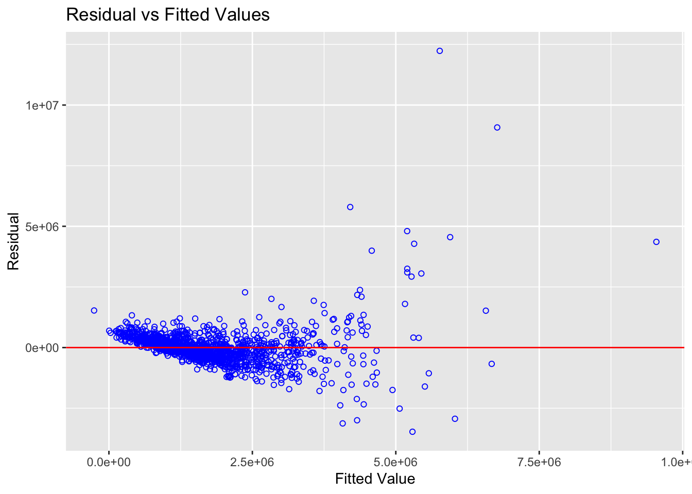
Test for Normality Assumption
# Visualise
ols_plot_resid_hist(condo.mlr1)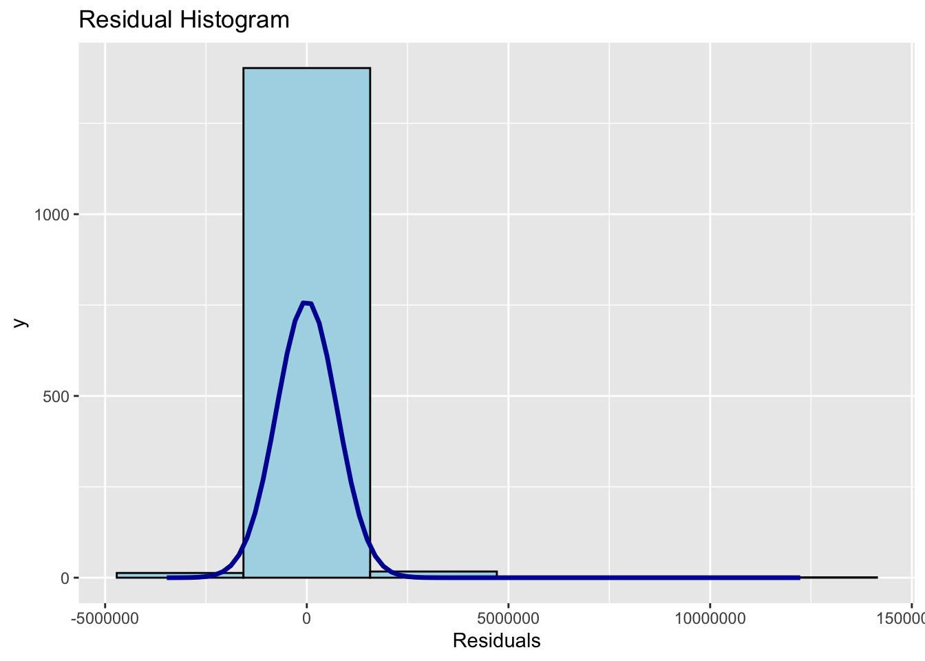
# For formal test stats
ols_test_normality(condo.mlr1)-----------------------------------------------
Test Statistic pvalue
-----------------------------------------------
Shapiro-Wilk 0.6856 0.0000
Kolmogorov-Smirnov 0.1366 0.0000
Cramer-von Mises 121.0768 0.0000
Anderson-Darling 67.9551 0.0000
-----------------------------------------------Test for spatial correlation
# Export and save as seperate df
mlr.output <- as.data.frame(condo.mlr1$residuals)
# Join new df
condo_resale.res.sf <- cbind(condo_resale.sf,
condo.mlr1$residuals) %>%
rename(`MLR_RES` = `condo.mlr1.residuals`)# Date conversion
condo_resale.sp <- as_Spatial(condo_resale.res.sf)
condo_resale.spclass : SpatialPointsDataFrame
features : 1436
extent : 14940.85, 43352.45, 24765.67, 48382.81 (xmin, xmax, ymin, ymax)
crs : +proj=tmerc +lat_0=1.36666666666667 +lon_0=103.833333333333 +k=1 +x_0=28001.642 +y_0=38744.572 +ellps=WGS84 +towgs84=0,0,0,0,0,0,0 +units=m +no_defs
variables : 23
names : POSTCODE, SELLING_PRICE, AREA_SQM, AGE, PROX_CBD, PROX_CHILDCARE, PROX_ELDERLYCARE, PROX_URA_GROWTH_AREA, PROX_HAWKER_MARKET, PROX_KINDERGARTEN, PROX_MRT, PROX_PARK, PROX_PRIMARY_SCH, PROX_TOP_PRIMARY_SCH, PROX_SHOPPING_MALL, ...
min values : 18965, 540000, 34, 0, 0.386916393, 0.004927023, 0.054508623, 0.214539508, 0.051817113, 0.004927023, 0.052779424, 0.029064164, 0.077106132, 0.077106132, 0, ...
max values : 828833, 1.8e+07, 619, 37, 19.18042832, 3.46572633, 3.949157205, 9.15540001, 5.374348075, 2.229045366, 3.48037319, 2.16104919, 3.928989144, 6.748192062, 3.477433767, ... Use visualization to eyeball and see if theres some kind of corr
tmap_mode("view")
tm_shape(mpsz_svy21)+
tmap_options(check.and.fix = TRUE) +
tm_polygons(alpha = 0.4) +
tm_shape(condo_resale.res.sf) +
tm_dots(col = "MLR_RES",
alpha = 0.6,
style="quantile") +
tm_view(set.zoom.limits = c(11,14))tmap_mode("plot")Since we can see clusters, do Moran I’s test
nb <- dnearneigh(coordinates(condo_resale.sp), 0, 1500, longlat = FALSE)
summary(nb)Neighbour list object:
Number of regions: 1436
Number of nonzero links: 66266
Percentage nonzero weights: 3.213526
Average number of links: 46.14624
Link number distribution:
1 3 5 7 9 10 11 12 13 14 15 16 17 18 19 20 21 22 23 24
3 3 9 4 3 15 10 19 17 45 19 5 14 29 19 6 35 45 18 47
25 26 27 28 29 30 31 32 33 34 35 36 37 38 39 40 41 42 43 44
16 43 22 26 21 11 9 23 22 13 16 25 21 37 16 18 8 21 4 12
45 46 47 48 49 50 51 52 53 54 55 56 57 58 59 60 61 62 63 64
8 36 18 14 14 43 11 12 8 13 12 13 4 5 6 12 11 20 29 33
65 66 67 68 69 70 71 72 73 74 75 76 77 78 79 80 81 82 83 84
15 20 10 14 15 15 11 16 12 10 8 19 12 14 9 8 4 13 11 6
85 86 87 88 89 90 91 92 93 94 95 96 97 98 99 100 101 102 103 104
4 9 4 4 4 6 2 16 9 4 5 9 3 9 4 2 1 2 1 1
105 106 107 108 109 110 112 116 125
1 5 9 2 1 3 1 1 1
3 least connected regions:
193 194 277 with 1 link
1 most connected region:
285 with 125 links# Convert to spatial weights
nb_lw <- nb2listw(nb, style = 'W')
summary(nb_lw)Characteristics of weights list object:
Neighbour list object:
Number of regions: 1436
Number of nonzero links: 66266
Percentage nonzero weights: 3.213526
Average number of links: 46.14624
Link number distribution:
1 3 5 7 9 10 11 12 13 14 15 16 17 18 19 20 21 22 23 24
3 3 9 4 3 15 10 19 17 45 19 5 14 29 19 6 35 45 18 47
25 26 27 28 29 30 31 32 33 34 35 36 37 38 39 40 41 42 43 44
16 43 22 26 21 11 9 23 22 13 16 25 21 37 16 18 8 21 4 12
45 46 47 48 49 50 51 52 53 54 55 56 57 58 59 60 61 62 63 64
8 36 18 14 14 43 11 12 8 13 12 13 4 5 6 12 11 20 29 33
65 66 67 68 69 70 71 72 73 74 75 76 77 78 79 80 81 82 83 84
15 20 10 14 15 15 11 16 12 10 8 19 12 14 9 8 4 13 11 6
85 86 87 88 89 90 91 92 93 94 95 96 97 98 99 100 101 102 103 104
4 9 4 4 4 6 2 16 9 4 5 9 3 9 4 2 1 2 1 1
105 106 107 108 109 110 112 116 125
1 5 9 2 1 3 1 1 1
3 least connected regions:
193 194 277 with 1 link
1 most connected region:
285 with 125 links
Weights style: W
Weights constants summary:
n nn S0 S1 S2
W 1436 2062096 1436 94.81916 5798.341# Perform Moran's I Test for spatial autocorr
lm.morantest(condo.mlr1, nb_lw)
Global Moran I for regression residuals
data:
model: lm(formula = SELLING_PRICE ~ AREA_SQM + AGE + PROX_CBD +
PROX_CHILDCARE + PROX_ELDERLYCARE + PROX_URA_GROWTH_AREA + PROX_MRT +
PROX_PARK + PROX_PRIMARY_SCH + PROX_SHOPPING_MALL + PROX_BUS_STOP +
NO_Of_UNITS + FAMILY_FRIENDLY + FREEHOLD, data = condo_resale.sf)
weights: nb_lw
Moran I statistic standard deviate = 24.366, p-value < 2.2e-16
alternative hypothesis: greater
sample estimates:
Observed Moran I Expectation Variance
1.438876e-01 -5.487594e-03 3.758259e-05 Hedonic Pricing Models with GWmodel
Fixed Bandwidth GWR model
# Determines optimal fixed bandwidth
bw.fixed <- bw.gwr(formula = SELLING_PRICE ~ AREA_SQM + AGE + PROX_CBD +
PROX_CHILDCARE + PROX_ELDERLYCARE + PROX_URA_GROWTH_AREA +
PROX_MRT + PROX_PARK + PROX_PRIMARY_SCH +
PROX_SHOPPING_MALL + PROX_BUS_STOP + NO_Of_UNITS +
FAMILY_FRIENDLY + FREEHOLD,
data=condo_resale.sp,
approach="CV",
kernel="gaussian",
adaptive=FALSE,
longlat=FALSE)Fixed bandwidth: 17660.96 CV score: 8.259118e+14
Fixed bandwidth: 10917.26 CV score: 7.970454e+14
Fixed bandwidth: 6749.419 CV score: 7.273273e+14
Fixed bandwidth: 4173.553 CV score: 6.300006e+14
Fixed bandwidth: 2581.58 CV score: 5.404958e+14
Fixed bandwidth: 1597.687 CV score: 4.857515e+14
Fixed bandwidth: 989.6077 CV score: 4.722431e+14
Fixed bandwidth: 613.7939 CV score: 1.379526e+16
Fixed bandwidth: 1221.873 CV score: 4.778717e+14
Fixed bandwidth: 846.0596 CV score: 4.791629e+14
Fixed bandwidth: 1078.325 CV score: 4.751406e+14
Fixed bandwidth: 934.7772 CV score: 4.72518e+14
Fixed bandwidth: 1023.495 CV score: 4.730305e+14
Fixed bandwidth: 968.6643 CV score: 4.721317e+14
Fixed bandwidth: 955.7206 CV score: 4.722072e+14
Fixed bandwidth: 976.6639 CV score: 4.721387e+14
Fixed bandwidth: 963.7202 CV score: 4.721484e+14
Fixed bandwidth: 971.7199 CV score: 4.721293e+14
Fixed bandwidth: 973.6083 CV score: 4.721309e+14
Fixed bandwidth: 970.5527 CV score: 4.721295e+14
Fixed bandwidth: 972.4412 CV score: 4.721296e+14
Fixed bandwidth: 971.2741 CV score: 4.721292e+14
Fixed bandwidth: 970.9985 CV score: 4.721293e+14
Fixed bandwidth: 971.4443 CV score: 4.721292e+14
Fixed bandwidth: 971.5496 CV score: 4.721293e+14
Fixed bandwidth: 971.3793 CV score: 4.721292e+14
Fixed bandwidth: 971.3391 CV score: 4.721292e+14
Fixed bandwidth: 971.3143 CV score: 4.721292e+14
Fixed bandwidth: 971.3545 CV score: 4.721292e+14
Fixed bandwidth: 971.3296 CV score: 4.721292e+14
Fixed bandwidth: 971.345 CV score: 4.721292e+14
Fixed bandwidth: 971.3355 CV score: 4.721292e+14
Fixed bandwidth: 971.3413 CV score: 4.721292e+14
Fixed bandwidth: 971.3377 CV score: 4.721292e+14
Fixed bandwidth: 971.34 CV score: 4.721292e+14
Fixed bandwidth: 971.3405 CV score: 4.721292e+14
Fixed bandwidth: 971.3396 CV score: 4.721292e+14
Fixed bandwidth: 971.3402 CV score: 4.721292e+14
Fixed bandwidth: 971.3398 CV score: 4.721292e+14
Fixed bandwidth: 971.34 CV score: 4.721292e+14
Fixed bandwidth: 971.3399 CV score: 4.721292e+14
Fixed bandwidth: 971.34 CV score: 4.721292e+14 We take the last result (is in metres)
# Calibrate gwr model
gwr.fixed <- gwr.basic(formula = SELLING_PRICE ~ AREA_SQM + AGE + PROX_CBD +
PROX_CHILDCARE + PROX_ELDERLYCARE + PROX_URA_GROWTH_AREA +
PROX_MRT + PROX_PARK + PROX_PRIMARY_SCH +
PROX_SHOPPING_MALL + PROX_BUS_STOP + NO_Of_UNITS +
FAMILY_FRIENDLY + FREEHOLD,
data=condo_resale.sp,
bw=bw.fixed,
kernel = 'gaussian',
longlat = FALSE)# Display model
gwr.fixed ***********************************************************************
* Package GWmodel *
***********************************************************************
Program starts at: 2023-03-27 12:02:59
Call:
gwr.basic(formula = SELLING_PRICE ~ AREA_SQM + AGE + PROX_CBD +
PROX_CHILDCARE + PROX_ELDERLYCARE + PROX_URA_GROWTH_AREA +
PROX_MRT + PROX_PARK + PROX_PRIMARY_SCH + PROX_SHOPPING_MALL +
PROX_BUS_STOP + NO_Of_UNITS + FAMILY_FRIENDLY + FREEHOLD,
data = condo_resale.sp, bw = bw.fixed, kernel = "gaussian",
longlat = FALSE)
Dependent (y) variable: SELLING_PRICE
Independent variables: AREA_SQM AGE PROX_CBD PROX_CHILDCARE PROX_ELDERLYCARE PROX_URA_GROWTH_AREA PROX_MRT PROX_PARK PROX_PRIMARY_SCH PROX_SHOPPING_MALL PROX_BUS_STOP NO_Of_UNITS FAMILY_FRIENDLY FREEHOLD
Number of data points: 1436
***********************************************************************
* Results of Global Regression *
***********************************************************************
Call:
lm(formula = formula, data = data)
Residuals:
Min 1Q Median 3Q Max
-3470778 -298119 -23481 248917 12234210
Coefficients:
Estimate Std. Error t value Pr(>|t|)
(Intercept) 527633.22 108183.22 4.877 1.20e-06 ***
AREA_SQM 12777.52 367.48 34.771 < 2e-16 ***
AGE -24687.74 2754.84 -8.962 < 2e-16 ***
PROX_CBD -77131.32 5763.12 -13.384 < 2e-16 ***
PROX_CHILDCARE -318472.75 107959.51 -2.950 0.003231 **
PROX_ELDERLYCARE 185575.62 39901.86 4.651 3.61e-06 ***
PROX_URA_GROWTH_AREA 39163.25 11754.83 3.332 0.000885 ***
PROX_MRT -294745.11 56916.37 -5.179 2.56e-07 ***
PROX_PARK 570504.81 65507.03 8.709 < 2e-16 ***
PROX_PRIMARY_SCH 159856.14 60234.60 2.654 0.008046 **
PROX_SHOPPING_MALL -220947.25 36561.83 -6.043 1.93e-09 ***
PROX_BUS_STOP 682482.22 134513.24 5.074 4.42e-07 ***
NO_Of_UNITS -245.48 87.95 -2.791 0.005321 **
FAMILY_FRIENDLY 146307.58 46893.02 3.120 0.001845 **
FREEHOLD 350599.81 48506.48 7.228 7.98e-13 ***
---Significance stars
Signif. codes: 0 '***' 0.001 '**' 0.01 '*' 0.05 '.' 0.1 ' ' 1
Residual standard error: 756000 on 1421 degrees of freedom
Multiple R-squared: 0.6507
Adjusted R-squared: 0.6472
F-statistic: 189.1 on 14 and 1421 DF, p-value: < 2.2e-16
***Extra Diagnostic information
Residual sum of squares: 8.120609e+14
Sigma(hat): 752522.9
AIC: 42966.76
AICc: 42967.14
BIC: 41731.39
***********************************************************************
* Results of Geographically Weighted Regression *
***********************************************************************
*********************Model calibration information*********************
Kernel function: gaussian
Fixed bandwidth: 971.34
Regression points: the same locations as observations are used.
Distance metric: Euclidean distance metric is used.
****************Summary of GWR coefficient estimates:******************
Min. 1st Qu. Median 3rd Qu.
Intercept -3.5988e+07 -5.1998e+05 7.6780e+05 1.7412e+06
AREA_SQM 1.0003e+03 5.2758e+03 7.4740e+03 1.2301e+04
AGE -1.3475e+05 -2.0813e+04 -8.6260e+03 -3.7784e+03
PROX_CBD -7.7047e+07 -2.3608e+05 -8.3599e+04 3.4646e+04
PROX_CHILDCARE -6.0097e+06 -3.3667e+05 -9.7426e+04 2.9007e+05
PROX_ELDERLYCARE -3.5001e+06 -1.5970e+05 3.1970e+04 1.9577e+05
PROX_URA_GROWTH_AREA -3.0170e+06 -8.2013e+04 7.0749e+04 2.2612e+05
PROX_MRT -3.5282e+06 -6.5836e+05 -1.8833e+05 3.6922e+04
PROX_PARK -1.2062e+06 -2.1732e+05 3.5383e+04 4.1335e+05
PROX_PRIMARY_SCH -2.2695e+07 -1.7066e+05 4.8472e+04 5.1555e+05
PROX_SHOPPING_MALL -7.2585e+06 -1.6684e+05 -1.0517e+04 1.5923e+05
PROX_BUS_STOP -1.4676e+06 -4.5207e+04 3.7601e+05 1.1664e+06
NO_Of_UNITS -1.3170e+03 -2.4822e+02 -3.0846e+01 2.5496e+02
FAMILY_FRIENDLY -2.2749e+06 -1.1140e+05 7.6214e+03 1.6107e+05
FREEHOLD -9.2067e+06 3.8074e+04 1.5169e+05 3.7528e+05
Max.
Intercept 112794435
AREA_SQM 21575
AGE 434203
PROX_CBD 2704604
PROX_CHILDCARE 1654086
PROX_ELDERLYCARE 38867861
PROX_URA_GROWTH_AREA 78515805
PROX_MRT 3124325
PROX_PARK 18122439
PROX_PRIMARY_SCH 4637517
PROX_SHOPPING_MALL 1529953
PROX_BUS_STOP 11342209
NO_Of_UNITS 12907
FAMILY_FRIENDLY 1720745
FREEHOLD 6073642
************************Diagnostic information*************************
Number of data points: 1436
Effective number of parameters (2trace(S) - trace(S'S)): 438.3807
Effective degrees of freedom (n-2trace(S) + trace(S'S)): 997.6193
AICc (GWR book, Fotheringham, et al. 2002, p. 61, eq 2.33): 42263.61
AIC (GWR book, Fotheringham, et al. 2002,GWR p. 96, eq. 4.22): 41632.36
BIC (GWR book, Fotheringham, et al. 2002,GWR p. 61, eq. 2.34): 42515.71
Residual sum of squares: 2.534069e+14
R-square value: 0.8909912
Adjusted R-square value: 0.8430418
***********************************************************************
Program stops at: 2023-03-27 12:03:00 Adaptive Bandwidth GWR Model
# Compute adaptive bandwidth
bw.adaptive <- bw.gwr(formula = SELLING_PRICE ~ AREA_SQM + AGE +
PROX_CBD + PROX_CHILDCARE + PROX_ELDERLYCARE +
PROX_URA_GROWTH_AREA + PROX_MRT + PROX_PARK +
PROX_PRIMARY_SCH + PROX_SHOPPING_MALL + PROX_BUS_STOP +
NO_Of_UNITS + FAMILY_FRIENDLY + FREEHOLD,
data=condo_resale.sp,
approach="CV",
kernel="gaussian",
adaptive=TRUE,
longlat=FALSE)Adaptive bandwidth: 895 CV score: 7.952401e+14
Adaptive bandwidth: 561 CV score: 7.667364e+14
Adaptive bandwidth: 354 CV score: 6.953454e+14
Adaptive bandwidth: 226 CV score: 6.15223e+14
Adaptive bandwidth: 147 CV score: 5.674373e+14
Adaptive bandwidth: 98 CV score: 5.426745e+14
Adaptive bandwidth: 68 CV score: 5.168117e+14
Adaptive bandwidth: 49 CV score: 4.859631e+14
Adaptive bandwidth: 37 CV score: 4.646518e+14
Adaptive bandwidth: 30 CV score: 4.422088e+14
Adaptive bandwidth: 25 CV score: 4.430816e+14
Adaptive bandwidth: 32 CV score: 4.505602e+14
Adaptive bandwidth: 27 CV score: 4.462172e+14
Adaptive bandwidth: 30 CV score: 4.422088e+14 # Use to calibrate model
gwr.adaptive <- gwr.basic(formula = SELLING_PRICE ~ AREA_SQM + AGE +
PROX_CBD + PROX_CHILDCARE + PROX_ELDERLYCARE +
PROX_URA_GROWTH_AREA + PROX_MRT + PROX_PARK +
PROX_PRIMARY_SCH + PROX_SHOPPING_MALL + PROX_BUS_STOP +
NO_Of_UNITS + FAMILY_FRIENDLY + FREEHOLD,
data=condo_resale.sp, bw=bw.adaptive,
kernel = 'gaussian',
adaptive=TRUE,
longlat = FALSE)# Display model
gwr.adaptive ***********************************************************************
* Package GWmodel *
***********************************************************************
Program starts at: 2023-03-27 12:03:13
Call:
gwr.basic(formula = SELLING_PRICE ~ AREA_SQM + AGE + PROX_CBD +
PROX_CHILDCARE + PROX_ELDERLYCARE + PROX_URA_GROWTH_AREA +
PROX_MRT + PROX_PARK + PROX_PRIMARY_SCH + PROX_SHOPPING_MALL +
PROX_BUS_STOP + NO_Of_UNITS + FAMILY_FRIENDLY + FREEHOLD,
data = condo_resale.sp, bw = bw.adaptive, kernel = "gaussian",
adaptive = TRUE, longlat = FALSE)
Dependent (y) variable: SELLING_PRICE
Independent variables: AREA_SQM AGE PROX_CBD PROX_CHILDCARE PROX_ELDERLYCARE PROX_URA_GROWTH_AREA PROX_MRT PROX_PARK PROX_PRIMARY_SCH PROX_SHOPPING_MALL PROX_BUS_STOP NO_Of_UNITS FAMILY_FRIENDLY FREEHOLD
Number of data points: 1436
***********************************************************************
* Results of Global Regression *
***********************************************************************
Call:
lm(formula = formula, data = data)
Residuals:
Min 1Q Median 3Q Max
-3470778 -298119 -23481 248917 12234210
Coefficients:
Estimate Std. Error t value Pr(>|t|)
(Intercept) 527633.22 108183.22 4.877 1.20e-06 ***
AREA_SQM 12777.52 367.48 34.771 < 2e-16 ***
AGE -24687.74 2754.84 -8.962 < 2e-16 ***
PROX_CBD -77131.32 5763.12 -13.384 < 2e-16 ***
PROX_CHILDCARE -318472.75 107959.51 -2.950 0.003231 **
PROX_ELDERLYCARE 185575.62 39901.86 4.651 3.61e-06 ***
PROX_URA_GROWTH_AREA 39163.25 11754.83 3.332 0.000885 ***
PROX_MRT -294745.11 56916.37 -5.179 2.56e-07 ***
PROX_PARK 570504.81 65507.03 8.709 < 2e-16 ***
PROX_PRIMARY_SCH 159856.14 60234.60 2.654 0.008046 **
PROX_SHOPPING_MALL -220947.25 36561.83 -6.043 1.93e-09 ***
PROX_BUS_STOP 682482.22 134513.24 5.074 4.42e-07 ***
NO_Of_UNITS -245.48 87.95 -2.791 0.005321 **
FAMILY_FRIENDLY 146307.58 46893.02 3.120 0.001845 **
FREEHOLD 350599.81 48506.48 7.228 7.98e-13 ***
---Significance stars
Signif. codes: 0 '***' 0.001 '**' 0.01 '*' 0.05 '.' 0.1 ' ' 1
Residual standard error: 756000 on 1421 degrees of freedom
Multiple R-squared: 0.6507
Adjusted R-squared: 0.6472
F-statistic: 189.1 on 14 and 1421 DF, p-value: < 2.2e-16
***Extra Diagnostic information
Residual sum of squares: 8.120609e+14
Sigma(hat): 752522.9
AIC: 42966.76
AICc: 42967.14
BIC: 41731.39
***********************************************************************
* Results of Geographically Weighted Regression *
***********************************************************************
*********************Model calibration information*********************
Kernel function: gaussian
Adaptive bandwidth: 30 (number of nearest neighbours)
Regression points: the same locations as observations are used.
Distance metric: Euclidean distance metric is used.
****************Summary of GWR coefficient estimates:******************
Min. 1st Qu. Median 3rd Qu.
Intercept -1.3487e+08 -2.4669e+05 7.7928e+05 1.6194e+06
AREA_SQM 3.3188e+03 5.6285e+03 7.7825e+03 1.2738e+04
AGE -9.6746e+04 -2.9288e+04 -1.4043e+04 -5.6119e+03
PROX_CBD -2.5330e+06 -1.6256e+05 -7.7242e+04 2.6624e+03
PROX_CHILDCARE -1.2790e+06 -2.0175e+05 8.7158e+03 3.7778e+05
PROX_ELDERLYCARE -1.6212e+06 -9.2050e+04 6.1029e+04 2.8184e+05
PROX_URA_GROWTH_AREA -7.2686e+06 -3.0350e+04 4.5869e+04 2.4613e+05
PROX_MRT -4.3781e+07 -6.7282e+05 -2.2115e+05 -7.4593e+04
PROX_PARK -2.9020e+06 -1.6782e+05 1.1601e+05 4.6572e+05
PROX_PRIMARY_SCH -8.6418e+05 -1.6627e+05 -7.7853e+03 4.3222e+05
PROX_SHOPPING_MALL -1.8272e+06 -1.3175e+05 -1.4049e+04 1.3799e+05
PROX_BUS_STOP -2.0579e+06 -7.1461e+04 4.1104e+05 1.2071e+06
NO_Of_UNITS -2.1993e+03 -2.3685e+02 -3.4699e+01 1.1657e+02
FAMILY_FRIENDLY -5.9879e+05 -5.0927e+04 2.6173e+04 2.2481e+05
FREEHOLD -1.6340e+05 4.0765e+04 1.9023e+05 3.7960e+05
Max.
Intercept 18758355
AREA_SQM 23064
AGE 13303
PROX_CBD 11346650
PROX_CHILDCARE 2892127
PROX_ELDERLYCARE 2465671
PROX_URA_GROWTH_AREA 7384059
PROX_MRT 1186242
PROX_PARK 2588497
PROX_PRIMARY_SCH 3381462
PROX_SHOPPING_MALL 38038564
PROX_BUS_STOP 12081592
NO_Of_UNITS 1010
FAMILY_FRIENDLY 2072414
FREEHOLD 1813995
************************Diagnostic information*************************
Number of data points: 1436
Effective number of parameters (2trace(S) - trace(S'S)): 350.3088
Effective degrees of freedom (n-2trace(S) + trace(S'S)): 1085.691
AICc (GWR book, Fotheringham, et al. 2002, p. 61, eq 2.33): 41982.22
AIC (GWR book, Fotheringham, et al. 2002,GWR p. 96, eq. 4.22): 41546.74
BIC (GWR book, Fotheringham, et al. 2002,GWR p. 61, eq. 2.34): 41914.08
Residual sum of squares: 2.528227e+14
R-square value: 0.8912425
Adjusted R-square value: 0.8561185
***********************************************************************
Program stops at: 2023-03-27 12:03:15 Visualise GWR Output
Convert SDF to sf
condo_resale.sf.adaptive <- st_as_sf(gwr.adaptive$SDF) %>%
st_transform(crs=3414)
condo_resale.sf.adaptive.svy21 <- st_transform(condo_resale.sf.adaptive, 3414)
condo_resale.sf.adaptive.svy21 Simple feature collection with 1436 features and 51 fields
Geometry type: POINT
Dimension: XY
Bounding box: xmin: 14940.85 ymin: 24765.67 xmax: 43352.45 ymax: 48382.81
Projected CRS: SVY21 / Singapore TM
First 10 features:
Intercept AREA_SQM AGE PROX_CBD PROX_CHILDCARE PROX_ELDERLYCARE
1 2050011.7 9561.892 -9514.634 -120681.9 319266.92 -393417.79
2 1633128.2 16576.853 -58185.479 -149434.2 441102.18 325188.74
3 3433608.2 13091.861 -26707.386 -259397.8 -120116.82 535855.81
4 234358.9 20730.601 -93308.988 2426853.7 480825.28 314783.72
5 2285804.9 6722.836 -17608.018 -316835.5 90764.78 -137384.61
6 -3568877.4 6039.581 -26535.592 327306.1 -152531.19 -700392.85
7 -2874842.4 16843.575 -59166.727 -983577.2 -177810.50 -122384.02
8 2038086.0 6905.135 -17681.897 -285076.6 70259.40 -96012.78
9 1718478.4 9580.703 -14401.128 105803.4 -657698.02 -123276.00
10 3457054.0 14072.011 -31579.884 -234895.4 79961.45 548581.04
PROX_URA_GROWTH_AREA PROX_MRT PROX_PARK PROX_PRIMARY_SCH
1 -159980.20 -299742.96 -172104.47 242668.03
2 -142290.39 -2510522.23 523379.72 1106830.66
3 -253621.21 -936853.28 209099.85 571462.33
4 -2679297.89 -2039479.50 -759153.26 3127477.21
5 303714.81 -44567.05 -10284.62 30413.56
6 -28051.25 733566.47 1511488.92 320878.23
7 1397676.38 -2745430.34 710114.74 1786570.95
8 269368.71 -14552.99 73533.34 53359.73
9 -361974.72 -476785.32 -132067.59 -40128.92
10 -150024.38 -1503835.53 574155.47 108996.67
PROX_SHOPPING_MALL PROX_BUS_STOP NO_Of_UNITS FAMILY_FRIENDLY FREEHOLD
1 300881.390 1210615.4 104.8290640 -9075.370 303955.6
2 -87693.378 1843587.2 -288.3441183 310074.664 396221.3
3 -126732.712 1411924.9 -9.5532945 5949.746 168821.7
4 -29593.342 7225577.5 -161.3551620 1556178.531 1212515.6
5 -7490.586 677577.0 42.2659674 58986.951 328175.2
6 258583.881 1086012.6 -214.3671271 201992.641 471873.1
7 -384251.210 5094060.5 -0.9212521 359659.512 408871.9
8 -39634.902 735767.1 30.1741069 55602.506 347075.0
9 276718.757 2815772.4 675.1615559 -30453.297 503872.8
10 -454726.822 2123557.0 -21.3044311 -100935.586 213324.6
y yhat residual CV_Score Stud_residual Intercept_SE AREA_SQM_SE
1 3000000 2886532 113468.16 0 0.38207013 516105.5 823.2860
2 3880000 3466801 413198.52 0 1.01433140 488083.5 825.2380
3 3325000 3616527 -291527.20 0 -0.83780678 963711.4 988.2240
4 4250000 5435482 -1185481.63 0 -2.84614670 444185.5 617.4007
5 1400000 1388166 11834.26 0 0.03404453 2119620.6 1376.2778
6 1320000 1516702 -196701.95 0 -0.72065801 28572883.7 2348.0091
7 3410000 3266881 143118.77 0 0.41291992 679546.6 893.5893
8 1420000 1431955 -11955.27 0 -0.03033109 2217773.1 1415.2604
9 2025000 1832799 192200.83 0 0.52018109 814281.8 943.8434
10 2550000 2223364 326635.53 0 1.10559735 2410252.0 1271.4073
AGE_SE PROX_CBD_SE PROX_CHILDCARE_SE PROX_ELDERLYCARE_SE
1 5889.782 37411.22 319111.1 120633.34
2 6226.916 23615.06 299705.3 84546.69
3 6510.236 56103.77 349128.5 129687.07
4 6010.511 469337.41 304965.2 127150.69
5 8180.361 410644.47 698720.6 327371.55
6 14601.909 5272846.47 1141599.8 1653002.19
7 8970.629 346164.20 530101.1 148598.71
8 8661.309 438035.69 742532.8 399221.05
9 11791.208 89148.35 704630.7 329683.30
10 9941.980 173532.77 500976.2 281876.74
PROX_URA_GROWTH_AREA_SE PROX_MRT_SE PROX_PARK_SE PROX_PRIMARY_SCH_SE
1 56207.39 185181.3 205499.6 152400.7
2 76956.50 281133.9 229358.7 165150.7
3 95774.60 275483.7 314124.3 196662.6
4 470762.12 279877.1 227249.4 240878.9
5 474339.56 363830.0 364580.9 249087.7
6 5496627.21 730453.2 1741712.0 683265.5
7 371692.97 375511.9 297400.9 344602.8
8 517977.91 423155.4 440984.4 261251.2
9 153436.22 285325.4 304998.4 278258.5
10 239182.57 571355.7 599131.8 331284.8
PROX_SHOPPING_MALL_SE PROX_BUS_STOP_SE NO_Of_UNITS_SE FAMILY_FRIENDLY_SE
1 109268.8 600668.6 218.1258 131474.7
2 98906.8 410222.1 208.9410 114989.1
3 119913.3 464156.7 210.9828 146607.2
4 177104.1 562810.8 361.7767 108726.6
5 301032.9 740922.4 299.5034 160663.7
6 2931208.6 1418333.3 602.5571 331727.0
7 249969.5 821236.4 532.1978 129241.2
8 351634.0 775038.4 338.6777 171895.1
9 289872.7 850095.5 439.9037 220223.4
10 265529.7 631399.2 259.0169 189125.5
FREEHOLD_SE Intercept_TV AREA_SQM_TV AGE_TV PROX_CBD_TV
1 115954.0 3.9720784 11.614302 -1.615447 -3.22582173
2 130110.0 3.3460017 20.087361 -9.344188 -6.32792021
3 141031.5 3.5629010 13.247868 -4.102368 -4.62353528
4 138239.1 0.5276150 33.577223 -15.524302 5.17080808
5 210641.1 1.0784029 4.884795 -2.152474 -0.77155660
6 374347.3 -0.1249043 2.572214 -1.817269 0.06207388
7 182216.9 -4.2305303 18.849348 -6.595605 -2.84136028
8 216649.4 0.9189786 4.879056 -2.041481 -0.65080678
9 220473.7 2.1104224 10.150733 -1.221345 1.18682383
10 206346.2 1.4343123 11.068059 -3.176418 -1.35360852
PROX_CHILDCARE_TV PROX_ELDERLYCARE_TV PROX_URA_GROWTH_AREA_TV PROX_MRT_TV
1 1.00048819 -3.2612693 -2.846248368 -1.61864578
2 1.47178634 3.8462625 -1.848971738 -8.92998600
3 -0.34404755 4.1319138 -2.648105057 -3.40075727
4 1.57665606 2.4756745 -5.691404992 -7.28705261
5 0.12990138 -0.4196596 0.640289855 -0.12249416
6 -0.13361179 -0.4237096 -0.005103357 1.00426206
7 -0.33542751 -0.8235874 3.760298131 -7.31116712
8 0.09462126 -0.2405003 0.520038994 -0.03439159
9 -0.93339393 -0.3739225 -2.359121712 -1.67102293
10 0.15961128 1.9461735 -0.627237944 -2.63204802
PROX_PARK_TV PROX_PRIMARY_SCH_TV PROX_SHOPPING_MALL_TV PROX_BUS_STOP_TV
1 -0.83749312 1.5923022 2.75358842 2.0154464
2 2.28192684 6.7019454 -0.88662640 4.4941192
3 0.66565951 2.9058009 -1.05686949 3.0419145
4 -3.34061770 12.9836105 -0.16709578 12.8383775
5 -0.02820944 0.1220998 -0.02488294 0.9145046
6 0.86781794 0.4696245 0.08821750 0.7656963
7 2.38773567 5.1844351 -1.53719231 6.2029165
8 0.16674816 0.2042469 -0.11271635 0.9493299
9 -0.43301073 -0.1442145 0.95462153 3.3123012
10 0.95831249 0.3290120 -1.71252687 3.3632555
NO_Of_UNITS_TV FAMILY_FRIENDLY_TV FREEHOLD_TV Local_R2
1 0.480589953 -0.06902748 2.621347 0.8846744
2 -1.380026395 2.69655779 3.045280 0.8899773
3 -0.045279967 0.04058290 1.197050 0.8947007
4 -0.446007570 14.31276425 8.771149 0.9073605
5 0.141120178 0.36714544 1.557983 0.9510057
6 -0.355762335 0.60891234 1.260522 0.9247586
7 -0.001731033 2.78285441 2.243875 0.8310458
8 0.089093858 0.32346758 1.602012 0.9463936
9 1.534793921 -0.13828365 2.285410 0.8380365
10 -0.082251138 -0.53369623 1.033819 0.9080753
geometry
1 POINT (22085.12 29951.54)
2 POINT (25656.84 34546.2)
3 POINT (23963.99 32890.8)
4 POINT (27044.28 32319.77)
5 POINT (41042.56 33743.64)
6 POINT (39717.04 32943.1)
7 POINT (28419.1 33513.37)
8 POINT (40763.57 33879.61)
9 POINT (23595.63 28884.78)
10 POINT (24586.56 33194.31)gwr.adaptive.output <- as.data.frame(gwr.adaptive$SDF)
condo_resale.sf.adaptive <- cbind(condo_resale.res.sf, as.matrix(gwr.adaptive.output))glimpse(condo_resale.sf.adaptive)Rows: 1,436
Columns: 77
$ POSTCODE <dbl> 118635, 288420, 267833, 258380, 467169, 466472…
$ SELLING_PRICE <dbl> 3000000, 3880000, 3325000, 4250000, 1400000, 1…
$ AREA_SQM <dbl> 309, 290, 248, 127, 145, 139, 218, 141, 165, 1…
$ AGE <dbl> 30, 32, 33, 7, 28, 22, 24, 24, 27, 31, 17, 22,…
$ PROX_CBD <dbl> 7.941259, 6.609797, 6.898000, 4.038861, 11.783…
$ PROX_CHILDCARE <dbl> 0.16597932, 0.28027246, 0.42922669, 0.39473543…
$ PROX_ELDERLYCARE <dbl> 2.5198118, 1.9333338, 0.5021395, 1.9910316, 1.…
$ PROX_URA_GROWTH_AREA <dbl> 6.618741, 7.505109, 6.463887, 4.906512, 6.4106…
$ PROX_HAWKER_MARKET <dbl> 1.76542207, 0.54507614, 0.37789301, 1.68259969…
$ PROX_KINDERGARTEN <dbl> 0.05835552, 0.61592412, 0.14120309, 0.38200076…
$ PROX_MRT <dbl> 0.5607188, 0.6584461, 0.3053433, 0.6910183, 0.…
$ PROX_PARK <dbl> 1.1710446, 0.1992269, 0.2779886, 0.9832843, 0.…
$ PROX_PRIMARY_SCH <dbl> 1.6340256, 0.9747834, 1.4715016, 1.4546324, 0.…
$ PROX_TOP_PRIMARY_SCH <dbl> 3.3273195, 0.9747834, 1.4715016, 2.3006394, 0.…
$ PROX_SHOPPING_MALL <dbl> 2.2102717, 2.9374279, 1.2256850, 0.3525671, 1.…
$ PROX_SUPERMARKET <dbl> 0.9103958, 0.5900617, 0.4135583, 0.4162219, 0.…
$ PROX_BUS_STOP <dbl> 0.10336166, 0.28673408, 0.28504777, 0.29872340…
$ NO_Of_UNITS <dbl> 18, 20, 27, 30, 30, 31, 32, 32, 32, 32, 34, 34…
$ FAMILY_FRIENDLY <dbl> 0, 0, 0, 0, 0, 1, 1, 0, 1, 1, 0, 0, 0, 0, 0, 0…
$ FREEHOLD <dbl> 1, 1, 1, 1, 1, 1, 1, 1, 1, 0, 1, 1, 1, 1, 1, 1…
$ LEASEHOLD_99YR <dbl> 0, 0, 0, 0, 0, 0, 0, 0, 0, 0, 0, 0, 0, 0, 0, 0…
$ LOG_SELLING_PRICE <dbl> 14.91412, 15.17135, 15.01698, 15.26243, 14.151…
$ MLR_RES <dbl> -1489099.55, 415494.57, 194129.69, 1088992.71,…
$ Intercept <dbl> 2050011.67, 1633128.24, 3433608.17, 234358.91,…
$ AREA_SQM.1 <dbl> 9561.892, 16576.853, 13091.861, 20730.601, 672…
$ AGE.1 <dbl> -9514.634, -58185.479, -26707.386, -93308.988,…
$ PROX_CBD.1 <dbl> -120681.94, -149434.22, -259397.77, 2426853.66…
$ PROX_CHILDCARE.1 <dbl> 319266.925, 441102.177, -120116.816, 480825.28…
$ PROX_ELDERLYCARE.1 <dbl> -393417.795, 325188.741, 535855.806, 314783.72…
$ PROX_URA_GROWTH_AREA.1 <dbl> -159980.203, -142290.389, -253621.206, -267929…
$ PROX_MRT.1 <dbl> -299742.96, -2510522.23, -936853.28, -2039479.…
$ PROX_PARK.1 <dbl> -172104.47, 523379.72, 209099.85, -759153.26, …
$ PROX_PRIMARY_SCH.1 <dbl> 242668.03, 1106830.66, 571462.33, 3127477.21, …
$ PROX_SHOPPING_MALL.1 <dbl> 300881.390, -87693.378, -126732.712, -29593.34…
$ PROX_BUS_STOP.1 <dbl> 1210615.44, 1843587.22, 1411924.90, 7225577.51…
$ NO_Of_UNITS.1 <dbl> 104.8290640, -288.3441183, -9.5532945, -161.35…
$ FAMILY_FRIENDLY.1 <dbl> -9075.370, 310074.664, 5949.746, 1556178.531, …
$ FREEHOLD.1 <dbl> 303955.61, 396221.27, 168821.75, 1212515.58, 3…
$ y <dbl> 3000000, 3880000, 3325000, 4250000, 1400000, 1…
$ yhat <dbl> 2886531.8, 3466801.5, 3616527.2, 5435481.6, 13…
$ residual <dbl> 113468.16, 413198.52, -291527.20, -1185481.63,…
$ CV_Score <dbl> 0, 0, 0, 0, 0, 0, 0, 0, 0, 0, 0, 0, 0, 0, 0, 0…
$ Stud_residual <dbl> 0.38207013, 1.01433140, -0.83780678, -2.846146…
$ Intercept_SE <dbl> 516105.5, 488083.5, 963711.4, 444185.5, 211962…
$ AREA_SQM_SE <dbl> 823.2860, 825.2380, 988.2240, 617.4007, 1376.2…
$ AGE_SE <dbl> 5889.782, 6226.916, 6510.236, 6010.511, 8180.3…
$ PROX_CBD_SE <dbl> 37411.22, 23615.06, 56103.77, 469337.41, 41064…
$ PROX_CHILDCARE_SE <dbl> 319111.1, 299705.3, 349128.5, 304965.2, 698720…
$ PROX_ELDERLYCARE_SE <dbl> 120633.34, 84546.69, 129687.07, 127150.69, 327…
$ PROX_URA_GROWTH_AREA_SE <dbl> 56207.39, 76956.50, 95774.60, 470762.12, 47433…
$ PROX_MRT_SE <dbl> 185181.3, 281133.9, 275483.7, 279877.1, 363830…
$ PROX_PARK_SE <dbl> 205499.6, 229358.7, 314124.3, 227249.4, 364580…
$ PROX_PRIMARY_SCH_SE <dbl> 152400.7, 165150.7, 196662.6, 240878.9, 249087…
$ PROX_SHOPPING_MALL_SE <dbl> 109268.8, 98906.8, 119913.3, 177104.1, 301032.…
$ PROX_BUS_STOP_SE <dbl> 600668.6, 410222.1, 464156.7, 562810.8, 740922…
$ NO_Of_UNITS_SE <dbl> 218.1258, 208.9410, 210.9828, 361.7767, 299.50…
$ FAMILY_FRIENDLY_SE <dbl> 131474.73, 114989.07, 146607.22, 108726.62, 16…
$ FREEHOLD_SE <dbl> 115954.0, 130110.0, 141031.5, 138239.1, 210641…
$ Intercept_TV <dbl> 3.9720784, 3.3460017, 3.5629010, 0.5276150, 1.…
$ AREA_SQM_TV <dbl> 11.614302, 20.087361, 13.247868, 33.577223, 4.…
$ AGE_TV <dbl> -1.6154474, -9.3441881, -4.1023685, -15.524301…
$ PROX_CBD_TV <dbl> -3.22582173, -6.32792021, -4.62353528, 5.17080…
$ PROX_CHILDCARE_TV <dbl> 1.000488185, 1.471786337, -0.344047555, 1.5766…
$ PROX_ELDERLYCARE_TV <dbl> -3.26126929, 3.84626245, 4.13191383, 2.4756745…
$ PROX_URA_GROWTH_AREA_TV <dbl> -2.846248368, -1.848971738, -2.648105057, -5.6…
$ PROX_MRT_TV <dbl> -1.61864578, -8.92998600, -3.40075727, -7.2870…
$ PROX_PARK_TV <dbl> -0.83749312, 2.28192684, 0.66565951, -3.340617…
$ PROX_PRIMARY_SCH_TV <dbl> 1.59230221, 6.70194543, 2.90580089, 12.9836104…
$ PROX_SHOPPING_MALL_TV <dbl> 2.753588422, -0.886626400, -1.056869486, -0.16…
$ PROX_BUS_STOP_TV <dbl> 2.0154464, 4.4941192, 3.0419145, 12.8383775, 0…
$ NO_Of_UNITS_TV <dbl> 0.480589953, -1.380026395, -0.045279967, -0.44…
$ FAMILY_FRIENDLY_TV <dbl> -0.06902748, 2.69655779, 0.04058290, 14.312764…
$ FREEHOLD_TV <dbl> 2.6213469, 3.0452799, 1.1970499, 8.7711485, 1.…
$ Local_R2 <dbl> 0.8846744, 0.8899773, 0.8947007, 0.9073605, 0.…
$ coords.x1 <dbl> 22085.12, 25656.84, 23963.99, 27044.28, 41042.…
$ coords.x2 <dbl> 29951.54, 34546.20, 32890.80, 32319.77, 33743.…
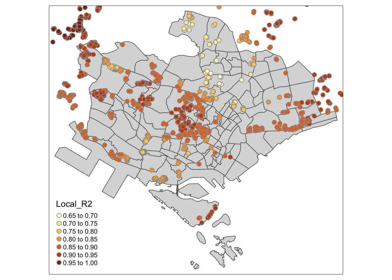
$ geometry <POINT [m]> POINT (22085.12 29951.54), POINT (25656.…Visualise local R2
tmap_mode("view")
tm_shape(mpsz_svy21)+
tm_polygons(alpha = 0.1) +
tm_shape(condo_resale.sf.adaptive) +
tm_dots(col = "Local_R2",
border.col = "gray60",
border.lwd = 1) +
tm_view(set.zoom.limits = c(11,14))Visualising coeff estimates
AREA_SQM_SE <- tm_shape(mpsz_svy21)+
tm_polygons(alpha = 0.1) +
tm_shape(condo_resale.sf.adaptive) +
tm_dots(col = "AREA_SQM_SE",
border.col = "gray60",
border.lwd = 1) +
tm_view(set.zoom.limits = c(11,14))
AREA_SQM_TV <- tm_shape(mpsz_svy21)+
tm_polygons(alpha = 0.1) +
tm_shape(condo_resale.sf.adaptive) +
tm_dots(col = "AREA_SQM_TV",
border.col = "gray60",
border.lwd = 1) +
tm_view(set.zoom.limits = c(11,14))
tmap_arrange(AREA_SQM_SE, AREA_SQM_TV,
asp=1, ncol=2,
sync = TRUE)Visualise by URA Planning Region
tmap_mode("plot")
tm_shape(mpsz_svy21[mpsz_svy21$REGION_N=="CENTRAL REGION", ])+
tm_polygons()+
tm_shape(condo_resale.sf.adaptive) +
tm_bubbles(col = "Local_R2",
size = 0.15,
border.col = "gray60",
border.lwd = 1)